XGBoost and LightGBM are currently very popular tree-based machine learning models, both demonstrating efficient performance. However, they have different characteristics in certain situations.
Simple Comparison of XGBoost and LightGBM
Training Speed
LightGBM has a significant advantage over XGBoost in terms of training speed. This is because LightGBM uses some efficient algorithms and data structures, such as the histogram algorithm and Gradient-based One-Side Sampling (GOSS), which allow LightGBM to train on large-scale datasets more quickly.
Memory Consumption
Due to the use of efficient algorithms and data structures, LightGBM has relatively low memory consumption. In contrast, XGBoost may require more memory when handling large-scale datasets.
Robustness
XGBoost is more robust when dealing with irregular data, such as missing values and outliers. LightGBM is relatively weaker in this aspect.
Accuracy
Under the same dataset and parameter settings, the accuracy of both models is roughly equivalent. However, in certain cases, XGBoost may perform better, such as when there are fewer features or when a smoother decision tree is needed.
Parameter Settings
XGBoost has more parameters that need to be adjusted according to the actual situation. LightGBM has relatively fewer parameters, and in most cases, the default parameters can be used.
Algorithm Comparison of XGBoost and LightGBM
XGBoost and LightGBM are both gradient boosting frameworks based on decision trees. Their core idea is to improve the model’s predictive capability by combining multiple weak learners. They have many similarities in implementation, but there are some clear differences in algorithms:
Split Point Selection Method
When constructing decision trees, XGBoost uses a greedy algorithm called the Exact Greedy Algorithm, which enumerates every feature’s possible values as split points, calculates the corresponding gain, and selects the split point with the maximum gain as the final split point.
LightGBM, on the other hand, uses a split point selection method based on Gradient-based One-Side Sampling (GOSS) and the histogram algorithm. It first pre-sorts the data, then divides the data into several histograms, each containing multiple data points. When searching for the optimal split point, LightGBM only selects a representative point (the maximum gradient value in the histogram) for calculation, significantly reducing the computational load.
Feature Parallel Processing
XGBoost divides the data by features and assigns each feature to different nodes for computation. This method can effectively increase training speed but requires additional communication and synchronization overhead.
LightGBM divides the data by rows and assigns each chunk to different nodes for computation. This method avoids communication and synchronization overhead but requires extra memory space.
Handling Missing Values
XGBoost automatically assigns missing values to the child node with the higher probability. This method may introduce some bias but is effective for datasets with many missing values.
LightGBM uses a method called Zero As Missing (ZAM), which treats all missing values as a special value and assigns them to one of the child nodes. This method can avoid bias but requires more memory space.
Training Speed
LightGBM has a significant advantage in training speed due to its use of GOSS and the histogram algorithm, which reduces computational load and memory consumption. In contrast, XGBoost’s computation speed is relatively slower, but it performs well on smaller datasets.
Electric Power Consumption Prediction
In today’s world, energy is one of the main discussion points. Accurately predicting energy consumption demand is crucial for any electricity company. Therefore, we will use energy prediction as an example to compare these two top models for tabular data.
We use the London energy dataset, which contains the energy consumption of 5,567 randomly selected households in London from November 2011 to February 2014. We will combine this dataset with the London weather dataset as auxiliary data to improve the model’s performance.
1. Preprocessing
The first thing we need to do in every project is to understand the data well and preprocess it when necessary:
 import pandas as pd
 import matplotlib.pyplot as plt

 df = pd.read_csv('london_energy.csv')
 print(df.isna().sum())
 df.head()
“LCLid” is the unique string identifying each household, “Date” is our time index, and “KWH” is the total kilowatt-hours spent on that date, with no missing values. Since we want to predict energy consumption in a general way rather than at the household level, we need to group the results by date and average the kilowatt-hours.
 df_avg_consumption = df.groupby('Date')['KWH'].mean()
 df_avg_consumption = pd.DataFrame({'date': df_avg_consumption.index.tolist(), 'consumption': df_avg_consumption.values.tolist()})
 df_avg_consumption['date'] = pd.to_datetime(df_avg_consumption['date'])
 print(f'From: {df_avg_consumption['date'].min()}')
 print(f'To: {df_avg_consumption['date'].max()}')
Create a line chart:
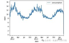
df_avg_consumption.plot(x='date', y='consumption')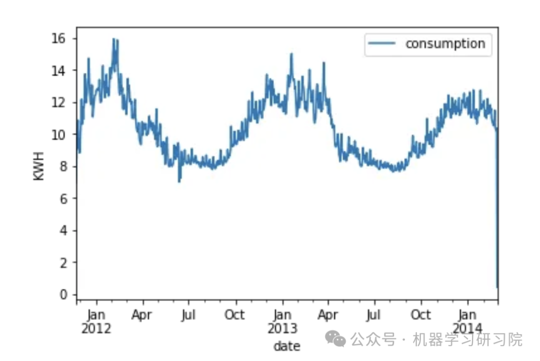
The seasonal features are very obvious. Energy demand is high in winter, while summer consumption is at its lowest. This behavior repeats every year in the dataset with different high and low values. Visualizing the fluctuations over a year:
df_avg_consumption.query('date > '2012-01-01' & date < '2013-01-01'').plot(x='date', y='consumption')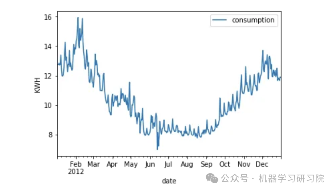
To train models like XGBoost and LightGBM, we need to create features ourselves. Currently, we only have one feature: the date. Therefore, we need to extract different features from the complete date, such as the day of the week, the day of the year, the month, and other dates:
 df_avg_consumption['day_of_week'] = df_avg_consumption['date'].dt.dayofweek
 df_avg_consumption['day_of_year'] = df_avg_consumption['date'].dt.dayofyear
 df_avg_consumption['month'] = df_avg_consumption['date'].dt.month
 df_avg_consumption['quarter'] = df_avg_consumption['date'].dt.quarter
 df_avg_consumption['year'] = df_avg_consumption['date'].dt.year

 df_avg_consumption.head()
'date' feature becomes redundant. However, before deleting it, we will use it to split the dataset into training and testing sets. Unlike traditional training, in time series, we cannot split the dataset randomly because the order of the data is very important. Therefore, for the testing set, we will only use the most recent six months of data. If the training set is larger, we can use the entire last year’s data as the testing set.
 training_mask = df_avg_consumption['date'] < '2013-07-28'
 training_data = df_avg_consumption.loc[training_mask]
 print(training_data.shape)

 testing_mask = df_avg_consumption['date'] >= '2013-07-28'
 testing_data = df_avg_consumption.loc[testing_mask]
 print(testing_data.shape)
Visualize the split between the training and testing sets:
 figure, ax = plt.subplots(figsize=(20, 5))
 training_data.plot(ax=ax, label='Training', x='date', y='consumption')
 testing_data.plot(ax=ax, label='Testing', x='date', y='consumption')
 plt.show()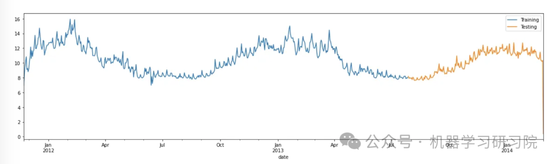
Now we can delete 'date' and create the training and testing sets:
 # Dropping unnecessary `date` column
 training_data = training_data.drop(columns=['date'])
 testing_dates = testing_data['date']
 testing_data = testing_data.drop(columns=['date'])

 X_train = training_data[['day_of_week', 'day_of_year', 'month', 'quarter', 'year']]
 y_train = training_data['consumption']

 X_test = testing_data[['day_of_week', 'day_of_year', 'month', 'quarter', 'year']]
 y_test = testing_data['consumption']
2. Train the Model
In this case, hyperparameter optimization will be done through grid search. Since it is a time series, we cannot use regular k-fold cross-validation. Scikit-learn provides the TimeSeriesSplit method, which can be used directly here.
 from xgboost import XGBRegressor
 import lightgbm as lgb
 from sklearn.model_selection import TimeSeriesSplit, GridSearchCV

 # XGBoost
 cv_split = TimeSeriesSplit(n_splits=4, test_size=100)
 model = XGBRegressor()
 parameters = {
    'max_depth': [3, 4, 6, 5, 10],
    'learning_rate': [0.01, 0.05, 0.1, 0.2, 0.3],
    'n_estimators': [100, 300, 500, 700, 900, 1000],
    'colsample_bytree': [0.3, 0.5, 0.7]
 }

 grid_search = GridSearchCV(estimator=model, cv=cv_split, param_grid=parameters)
 grid_search.fit(X_train, y_train)
For LightGB, the code is as follows:
 # LGBM
 cv_split = TimeSeriesSplit(n_splits=4, test_size=100)
 model = lgb.LGBMRegressor()
 parameters = {
    'max_depth': [3, 4, 6, 5, 10],
    'num_leaves': [10, 20, 30, 40, 100, 120],
    'learning_rate': [0.01, 0.05, 0.1, 0.2, 0.3],
    'n_estimators': [50, 100, 300, 500, 700, 900, 1000],
    'colsample_bytree': [0.3, 0.5, 0.7, 1]
 }

 grid_search = GridSearchCV(estimator=model, cv=cv_split, param_grid=parameters)
 grid_search.fit(X_train, y_train)
3. Evaluation
To evaluate the best estimator on the testing set, we will calculate: Mean Absolute Error (MAE), Mean Squared Error (MSE), and Mean Absolute Percentage Error (MAPE). Each metric provides a different perspective on the actual performance of the trained model. We will also plot a line chart to better visualize the model’s performance.
 from sklearn.metrics import mean_absolute_error, mean_absolute_percentage_error,\
  mean_squared_error

 def evaluate_model(y_test, prediction):
  print(f'MAE: {mean_absolute_error(y_test, prediction)}')
  print(f'MSE: {mean_squared_error(y_test, prediction)}')
  print(f'MAPE: {mean_absolute_percentage_error(y_test, prediction)}')

 def plot_predictions(testing_dates, y_test, prediction):
  df_test = pd.DataFrame({'date': testing_dates, 'actual': y_test, 'prediction': prediction })
  figure, ax = plt.subplots(figsize=(10, 5))
  df_test.plot(ax=ax, label='Actual', x='date', y='actual')
  df_test.plot(ax=ax, label='Prediction', x='date', y='prediction')
  plt.legend(['Actual', 'Prediction'])
  plt.show()
Then we run the following code for validation:
# Evaluating GridSearch results
prediction = grid_search.predict(X_test)
plot_predictions(testing_dates, y_test, prediction)
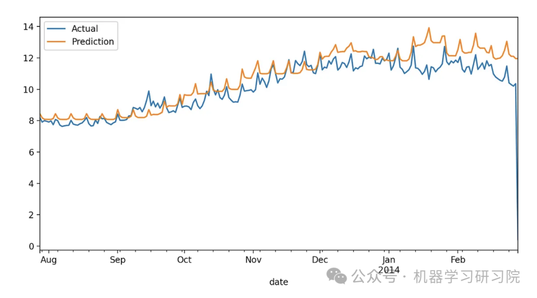
evaluate_model(y_test, prediction)XGB:
LightGBM:
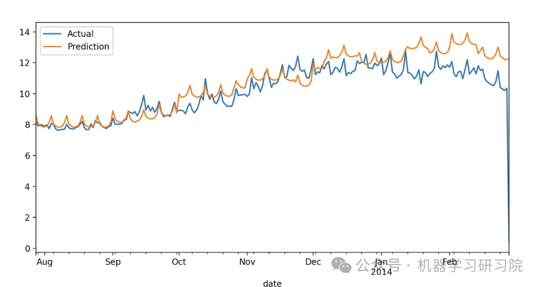
From the graphs, we can see that XGBoost can predict winter energy consumption more accurately. However, to quantify and compare performance, we calculate the error metrics. By looking at the table below, it is evident that XGBoost outperforms LightGBM in all cases.
| Metric | XGBoost | LightGBM |
|---|---|---|
| MAE | 0.7004574304534286 | 0.7641422971418719 |
| MSE | 1.2969848396218415 | 1.516060641278837 |
| MAPE | 0.19009300735560086 | 0.19830648942066428 |
Using External Auxiliary Weather Data
The model performs well, but can we improve it further? To achieve better results, many different techniques and tricks can be employed. One of them is to use auxiliary features that are directly or indirectly related to energy consumption. For example, weather data can play a decisive role in predicting energy demand. This is why we chose to use the weather data from the London weather dataset.
First, let’s take a look at the structure of the data:
 df_weather = pd.read_csv('london_weather.csv')
 print(df_weather.isna().sum())
 df_weather.head()
This dataset has various missing values that need to be filled. Filling missing values is not a simple task, as different situations require different filling methods. For our weather data, daily values depend on the previous few days and the next day, so we can fill these values through interpolation. Additionally, we need to convert the ‘date’ column to ‘datetime’ and then merge the two DataFrames to obtain an enhanced complete dataset.
 # Parsing dates
 df_weather['date'] = pd.to_datetime(df_weather['date'], format='%Y%m%d')

 # Filling missing values through interpolation
 df_weather = df_weather.interpolate(method='ffill')

 # Enhancing consumption dataset with weather information
 df_avg_consumption = df_avg_consumption.merge(df_weather, how='inner', on='date')
 df_avg_consumption.head()
After generating the enhanced dataset, we must rerun the splitting process to obtain new 'training_data' and 'testing_data'.
 # Dropping unnecessary `date` column
 training_data = training_data.drop(columns=['date'])
 testing_dates = testing_data['date']
 testing_data = testing_data.drop(columns=['date'])

 X_train = training_data[['day_of_week', 'day_of_year', 'month', 'quarter', 'year',\
                          'cloud_cover', 'sunshine', 'global_radiation', 'max_temp',\
                          'mean_temp', 'min_temp', 'precipitation', 'pressure',\
                          'snow_depth']]
 y_train = training_data['consumption']


 X_test = testing_data[['day_of_week', 'day_of_year', 'month', 'quarter', 'year',\
                          'cloud_cover', 'sunshine', 'global_radiation', 'max_temp',\
                          'mean_temp', 'min_temp', 'precipitation', 'pressure',\
                          'snow_depth']]
 y_test = testing_data['consumption']
The training steps do not need to be changed. After training the model on the new dataset, we obtain the following results:
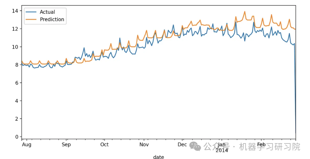
XGBoost
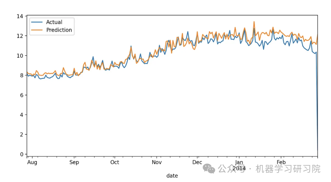
LightGBM
Integrating the tables above:
| Metric | XGBoost | XGBoost(Weather) | LightGBM | LightGBM(Weather) |
|---|---|---|---|---|
| MAE | 0.7004574304534286 | 0.3867829815893989 | 0.7641422971418719 | 0.44328143924280733 |
| MSE | 1.2969848396218415 | 0.8218867663903024 | 1.516060641278837 | 0.8729799405489558 |
| MAPE | 0.19009300735560086 | 0.16035702481330552 | 0.19830648942066428 | 0.1672249593119879 |
We see that weather data significantly improves the performance of both models. Especially in the XGBoost scenario, MAE decreased by nearly 44%, and MAPE dropped from 19% to 16%. For LightGBM, MAE decreased by 42%, and MAPE dropped from 19.8% to 16.7%.
Conclusion
XGBoost and LightGBM are both excellent gradient boosting frameworks, each with unique advantages and disadvantages. The choice of which algorithm to use should depend on the specific application scenario and the characteristics of the dataset. If the dataset has many missing values, XGBoost may be a better choice. If handling large-scale datasets and seeking faster training speed is a priority, LightGBM should be selected. If model interpretability and feature importance evaluation are needed, XGBoost provides better methods for assessing feature importance. If a more robust model is required, XGBoost should be prioritized.
In this article, we also introduced a method to improve the model by using additional data. By adding auxiliary data that we consider relevant, we can significantly enhance the model’s performance.
Additionally, we can explore lag features or try different hyperparameter optimization techniques (such as random search or Bayesian optimization) as attempts to improve performance. If you have any new results, feel free to leave a comment.
Here are the links to the two datasets:
https://www.kaggle.com/datasets/emmanuelfwerr/london-homes-energy-data https://www.kaggle.com/datasets/emmanuelfwerr/london-weather-data