
This article will explain in detail the introduction, functionality, and value ranges of the ten most commonly used hyperparameters in XGBoost, and how to use Optuna for hyperparameter tuning.

For XGBoost, the default hyperparameters work fine, but if you want to achieve the best performance, you need to adjust some hyperparameters to match your data. The following parameters are very important for XGBoost:
-
eta -
num_boost_round -
max_depth -
subsample -
colsample_bytree -
gamma -
min_child_weight -
lambda -
alpha
XGBoost has two ways to call its API: one is the native API that we commonly use, and the other is the Scikit-learn compatible API, which integrates seamlessly with the Sklearn ecosystem. Here, we focus only on the native API (which is the most common), but here is a list to help you compare the parameters of the two APIs, just in case you need it in the future:
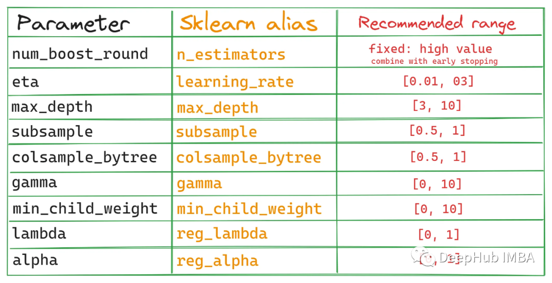
If you want to use hyperparameter tuning tools other than Optuna, you can refer to this table. The following figure shows the interactions between these parameters:
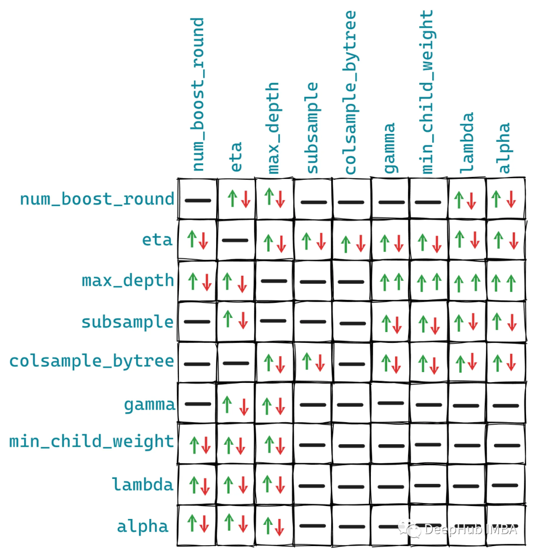
These relationships are not fixed, but the general situation is as shown in the figure above, as some other parameters may have additional effects on our ten parameters.
1. objective
This is the training objective of our model.
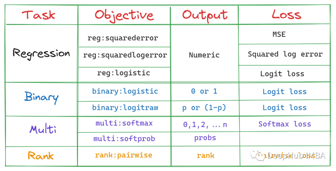
The simplest explanation is that this parameter specifies what our model is supposed to do, which affects the types of decision trees and the loss function.
2. num_boost_round – n_estimators
num_boost_round specifies the number of decision trees (usually referred to as base learners in XGBoost) to be generated during training. The default value is 100, but this is far from sufficient for today’s large datasets.
Increasing this parameter can generate more trees, but as the model becomes more complex, the chances of overfitting also significantly increase.
A trick learned from Kaggle is to set a high value for num_boost_round, such as 100,000, and use early stopping to obtain the best version.
In each boosting round, XGBoost generates more decision trees to improve the overall score of the previous decision tree. That’s why it’s called boosting. This process continues until num_boost_round rounds are completed, regardless of whether there is an improvement compared to the previous round.
However, by using early stopping techniques, we can stop training when the validation metric does not improve, which not only saves time but also prevents overfitting.
With this trick, we do not even need to tune num_boost_round. Here’s how it looks in code:
 # Define the rest of the params
 params = {...}

 # Build the train/validation sets
 dtrain_final = xgb.DMatrix(X_train, label=y_train)
 dvalid_final = xgb.DMatrix(X_valid, label=y_valid)

 bst_final = xgb.train(
     params,
     dtrain_final,
     num_boost_round=100000 # Set a high number
     evals=[(dvalid_final, "validation")],
     early_stopping_rounds=50, # Enable early stopping
     verbose_eval=False,
 )
The code above makes XGBoost generate 100k decision trees, but due to the use of early stopping, it will stop when the validation score does not improve in the last 50 rounds. Generally, the number of trees ranges from 5000 to 10000. Controlling num_boost_round is also one of the biggest factors affecting the run time of the training process, as more trees require more resources.
3. eta – learning_rate
In each round, all existing trees return a prediction for the given input. For example, five trees might return the following predictions for sample N:
Tree 1: 0.57 Tree 2: 0.9 Tree 3: 4.25 Tree 4: 6.4 Tree 5: 2.1To return the final prediction, these outputs need to be aggregated, but before that, XGBoost uses a parameter called eta or learning rate to shrink or scale them. The scaled final output is:
output = eta * (0.57 + 0.9 + 4.25 + 6.4 + 2.1)A large learning rate assigns greater weight to each tree’s contribution in the ensemble, but this can lead to overfitting/instability and speed up training time. A lower learning rate suppresses each tree’s contribution, making the learning process slower but more robust. This regularization effect of the learning rate parameter is particularly useful for complex and noisy datasets.
The learning rate is inversely related to other parameters like num_boost_round, max_depth, subsample, and colsample_bytree. A lower learning rate requires higher values of these parameters, and vice versa. However, in general, there is no need to worry about the interactions between these parameters, as we will use automated tuning to find the best combination.
4. subsample and colsample_bytree
Subsampling (subsample) introduces more randomness into the training, which helps combat overfitting.
Subsample = 0.7 means that each decision tree in the ensemble will be trained on a randomly selected 70% of the available data. A value of 1.0 indicates that all rows will be used (no subsampling).
Similar to subsample, there is also colsample_bytree. As the name suggests, colsample_bytree controls the proportion of features that each decision tree will use. Colsample_bytree = 0.8 means that each tree will use 80% of the available features (columns) randomly.
Tuning these two parameters can control the trade-off between bias and variance. Using smaller values reduces the correlation between trees, increases diversity in the ensemble, helps improve generalization, and reduces overfitting.
However, they may introduce more noise, increasing the model’s bias. Using larger values increases the correlation between trees, decreases diversity, and may lead to overfitting.
5. max_depth
The maximum depth (max_depth) controls the maximum number of layers a decision tree can reach during training.
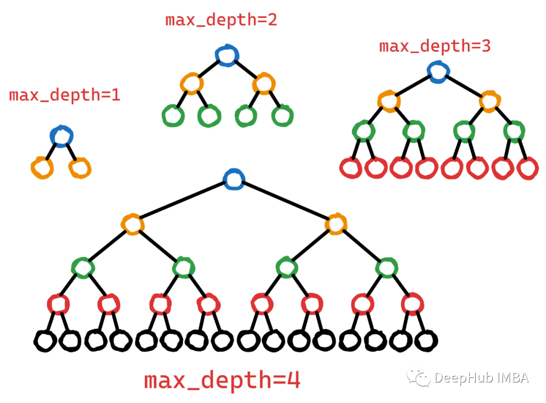
Deeper trees can capture more complex interactions between features. However, deeper trees also have a higher risk of overfitting, as they can memorize noise or irrelevant patterns in the training data. To control this complexity, max_depth can be limited, resulting in shallower, simpler trees that capture more general patterns.
The max_depth value can balance complexity and generalization well.
6, 7. alpha, lambda
These two parameters are mentioned together because alpha (L1) and lambda (L2) are two regularization parameters that help prevent overfitting.
Unlike other regularization parameters, they can shrink the weights of unimportant or irrelevant features to 0 (especially alpha), resulting in a model with fewer features, thus reducing complexity.
The effects of alpha and lambda may be influenced by other parameters such as max_depth, subsample, and colsample_bytree. Higher alpha or lambda values may require tuning other parameters to compensate for the increased regularization. For example, a higher alpha value may benefit from a larger subsample value, as this can maintain model diversity and prevent underfitting.
8. gamma
If you have read the XGBoost documentation, it states that gamma is:
The minimum loss reduction required to make a further partition on a leaf node of the tree.
English original: the minimum loss reduction required to make a further partition on a leaf node of the tree.
I think that except for the person who wrote this sentence, no one else can understand it. Let’s see what it really is; here’s a two-layer decision tree:
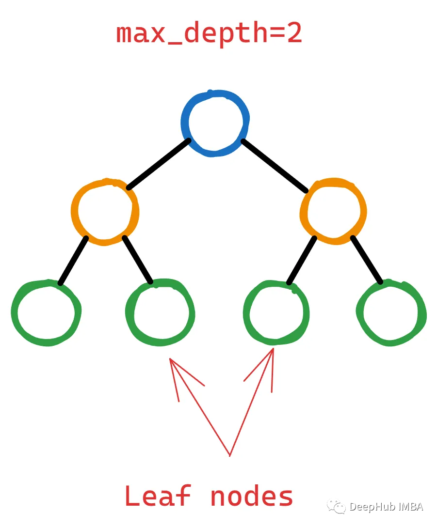
To justify adding more layers to the tree by splitting leaf nodes, XGBoost should compute whether this operation can significantly reduce the loss function.
But “how significant is significant?” That’s gamma—it serves as a threshold to determine whether a leaf node should be further split.
If the reduction in the loss function (commonly referred to as gain) after the potential split is less than the chosen gamma, the split is not performed. This means the leaf node will remain unchanged, and the tree will not grow from that point.
So the tuning goal is to find the best split that leads to the maximum reduction in the loss function, which means improved model performance.
9. min_child_weight
XGBoost starts the initial training process with a single decision tree that has a single root node. This node contains all training instances (rows). As XGBoost selects potential features and splitting criteria to minimize loss, deeper nodes will contain fewer and fewer instances.
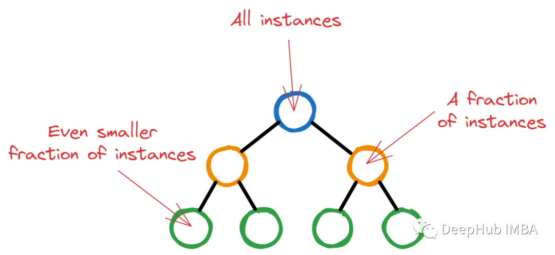
If XGBoost runs arbitrarily, the tree may grow to the point where there are only a few irrelevant instances in the last node. This situation is highly undesirable, as it is the very definition of overfitting.
Therefore, XGBoost sets a threshold for the minimum number of instances that must be present in a node to continue splitting. By weighting all instances in the node and finding the total weight, if this final weight is less than min_child_weight, the split stops, and the node becomes a leaf node.
The above explanation is a simplified version of the entire process, as we mainly introduce its concept.
Summary
That’s our explanation of these 10 important hyperparameters. If you want to delve deeper, there is still much to learn. Therefore, it is recommended to give ChatGPT the following two prompts:
 1) Explain the {parameter_name} XGBoost parameter in detail and how to choose values for it wisely.

 2) Describe how {parameter_name} fits into the step-by-step tree-building process of XGBoost.
It will definitely explain it better than I can, right?
Finally, if you also use Optuna for tuning, please refer to the following GIST:
https://gist.github.com/BexTuychiev/823df08d2e3760538e9b931d38439a68
Author: Bex T.