XGBoost: A Powerful Algorithm Model

Core Points:From Principles to Cases, A Complete Summary of XGBoost!

Hello, I am Cos Dazhuang~

Recently, many people have been messaging about XGBoost, feeling it’s very useful but still somewhat unclear.

Today, we will clarify it from principles, derivation of formulas, to a practical case at the end, hoping it helps!

In simple terms, XGBoost is an efficient, flexible, and scalable gradient boosting tree (GBDT) library, widely used for regression, classification, and ranking problems. XGBoost significantly enhances model performance and computation speed by introducing second-order derivative optimization, regularization, and distributed computing. It performs exceptionally well in many data science competitions and is very powerful!

As Usual: If you think recent articles are good, feel free to like and share~

Let’s take a look together~

XGBoost Principles

Basic Concept of Gradient Boosting Trees

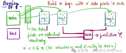
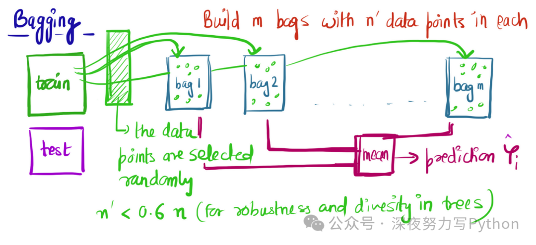
Gradient Boosting is an iterative machine learning method that combines multiple weak learners (usually decision trees) to gradually improve model performance. The core idea is to train a new weak learner to correct the errors of the previous model at each iteration.

The basic steps of gradient boosting are:

1. Initialize the model, usually using the mean of the training data.
2. For each iteration:

• Calculate the residuals of the current model, where is the target value and is the current model’s prediction.
• Train a new decision tree to fit the residuals.
• Update the model, where is the newly trained decision tree and is the learning rate.

Innovations of XGBoost

XGBoost has made several improvements to the traditional gradient boosting framework:

• Regularization: XGBoost introduces a regularization term in the objective function to prevent overfitting.
• Taylor Expansion of Loss Function: Optimizing using the second-order Taylor expansion of the loss function enhances computational efficiency.
• Column Subsampling: Similar to random forests, XGBoost randomly samples features when training each tree, improving the model’s generalization ability.
• Efficient Split Finding Algorithm: Accelerates the training process using a cache-aware block structure.

The objective function of XGBoost is:

Where:

• is the training error (such as squared error, log loss, etc.).
• is the regularization term for the tree, which includes the tree’s complexity and the weights of the leaf nodes.

By performing a second-order Taylor expansion of the loss function, we can obtain an approximate optimization objective:

Where is the first derivative and is the second derivative.

By optimizing the above, we can efficiently train a new decision tree.

Practical Case

Next, we will use the “Titanic Survivor Prediction” dataset as a case study.

This is a classic classification problem, very suitable for demonstrating the application of XGBoost. Below are the complete steps, including data loading, preprocessing, model training, evaluation, and visualization.

In the code, the Titanic survivor prediction dataset titanic.csv is involved. If needed, click on the business card and reply with “dataset”!

1. Data Preparation

First, load and process the data:

import pandas as pd
from sklearn.model_selection import train_test_split
from sklearn.preprocessing import StandardScaler
import xgboost as xgb
import matplotlib.pyplot as plt
import seaborn as sns

# Read data
data = pd.read_csv('titanic.csv')

# View data overview
print(data.info())
print(data.describe())

# Select features and target variable
features = data.drop(['Survived', 'Name', 'Ticket', 'Cabin'], axis=1)
target = data['Survived']

# Fill missing values
features['Age'] = features['Age'].fillna(features['Age'].mean())
features['Embarked'] = features['Embarked'].fillna(features['Embarked'].mode()[0])

# Convert categorical variables
features = pd.get_dummies(features)

# Data standardization
scaler = StandardScaler()
features = scaler.fit_transform(features)

# Split training and test sets
X_train, X_test, y_train, y_test = train_test_split(features, target, test_size=0.2, random_state=42)

2. Model Training

Use XGBoost for model training:

# Convert data format
dtrain = xgb.DMatrix(X_train, label=y_train)
dtest = xgb.DMatrix(X_test, label=y_test)

# Set parameters
params = {
    'objective': 'binary:logistic',
    'learning_rate': 0.1,
    'max_depth': 6,
    'min_child_weight': 1,
    'subsample': 0.8,
    'colsample_bytree': 0.8,
    'n_estimators': 100
}

# Train model
model = xgb.train(params, dtrain, num_boost_round=100, evals=[(dtest, 'test')], early_stopping_rounds=10)

# Predict
y_pred = model.predict(dtest)
y_pred_binary = [1 if pred > 0.5 else 0 for pred in y_pred]

3. Model Evaluation

Evaluate the model using accuracy:

from sklearn.metrics import accuracy_score, confusion_matrix, classification_report

# Calculate accuracy
accuracy = accuracy_score(y_test, y_pred_binary)
print(f'Accuracy: {accuracy:.4f}')

# Confusion matrix
conf_matrix = confusion_matrix(y_test, y_pred_binary)
print('Confusion Matrix:')
print(conf_matrix)

# Classification report
class_report = classification_report(y_test, y_pred_binary)
print('Classification Report:')
print(class_report)

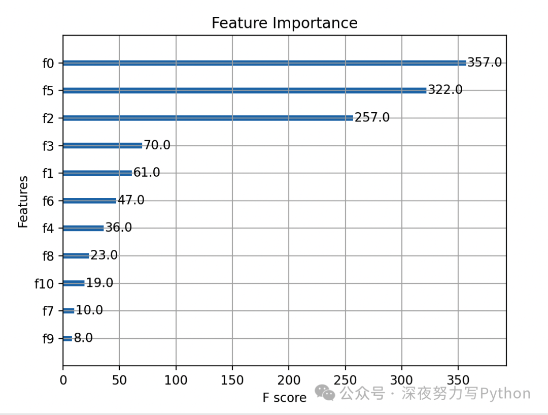
4. Feature Importance Visualization

Draw the feature importance graph:

# Feature importance
xgb.plot_importance(model)
plt.title('Feature Importance')
plt.show()

5. Hyperparameter Tuning

Use grid search for hyperparameter tuning:

from sklearn.model_selection import GridSearchCV
from xgboost import XGBClassifier

# Define parameter grid
param_grid = {
    'learning_rate': [0.01, 0.05, 0.1],
    'max_depth': [3, 5, 7],
    'min_child_weight': [1, 3, 5],
    'subsample': [0.6, 0.8, 1.0],
    'colsample_bytree': [0.6, 0.8, 1.0],
    'n_estimators': [100, 200, 300]
}

# Initialize model
xgb_model = XGBClassifier(objective='binary:logistic')

# Grid search
grid_search = GridSearchCV(estimator=xgb_model, param_grid=param_grid, scoring='accuracy', cv=3, verbose=1, n_jobs=-1)
grid_search.fit(X_train, y_train)

# Best parameters
print("Best parameters found: ", grid_search.best_params_)
print("Best accuracy found: ", grid_search.best_score_)

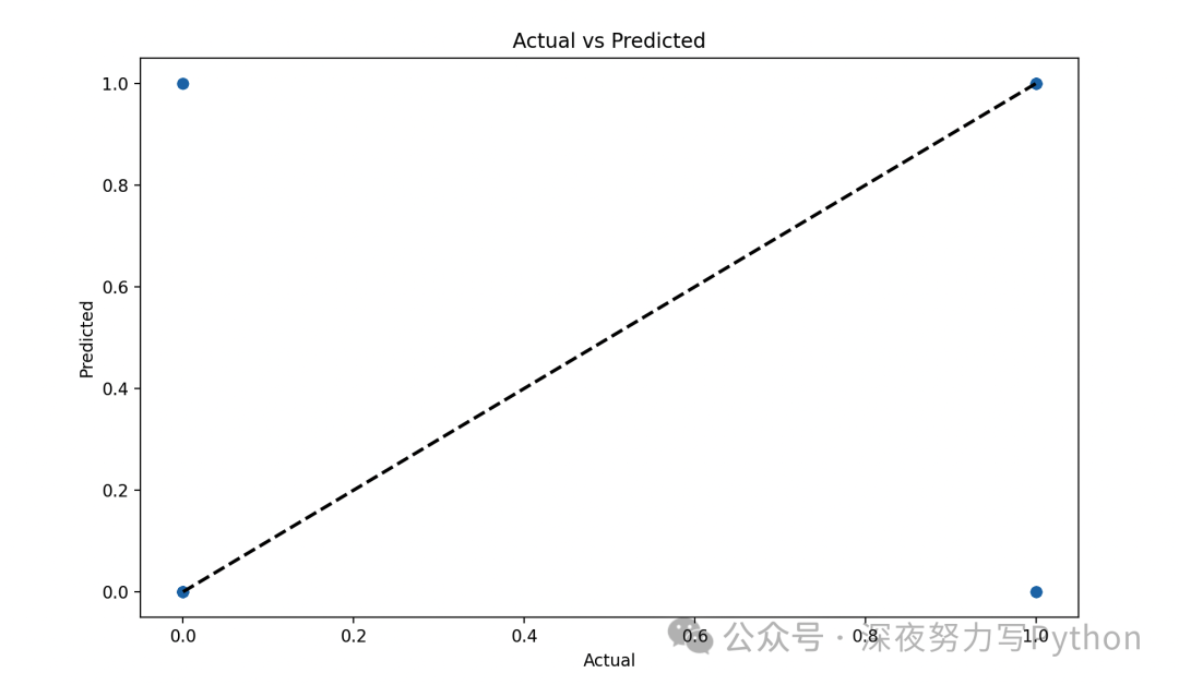
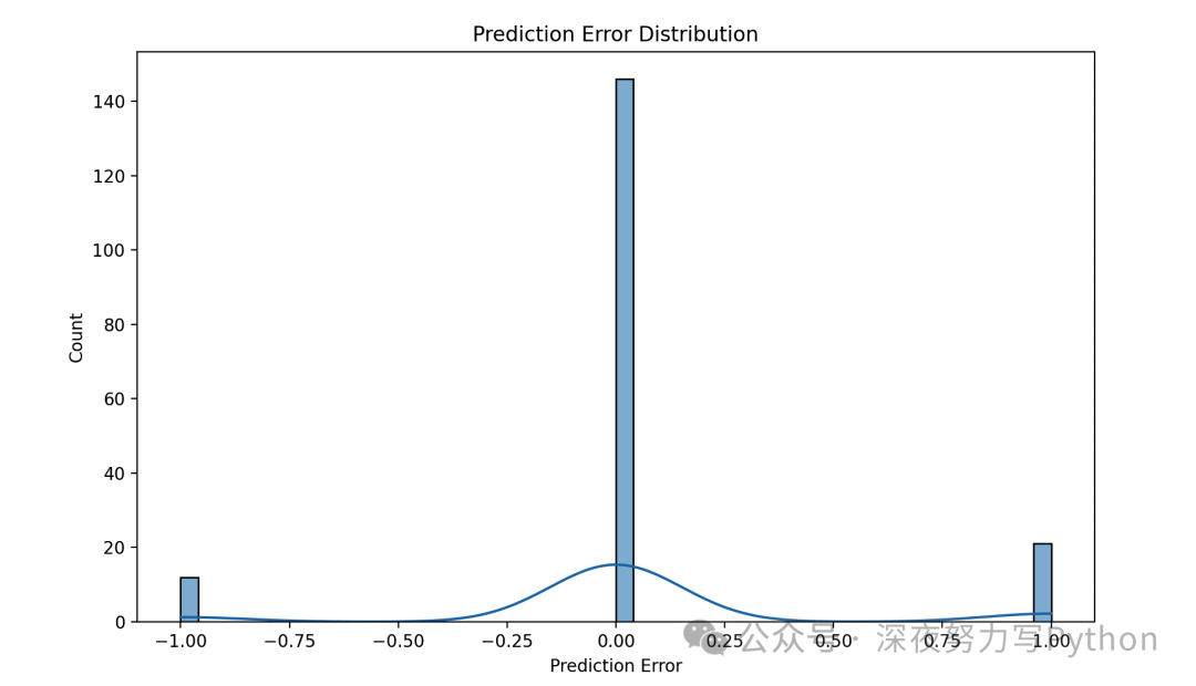
6. Result Visualization

Draw comparison graphs of predicted results and actual values, as well as error distribution graphs:

# Draw comparison graph of actual and predicted values
plt.figure(figsize=(10, 6))
plt.scatter(y_test, y_pred_binary, alpha=0.3)
plt.plot([0, 1], [0, 1], 'k--', lw=2)
plt.xlabel('Actual')
plt.ylabel('Predicted')
plt.title('Actual vs Predicted')
plt.show()

# Draw error distribution graph
errors = y_test - y_pred_binary
plt.figure(figsize=(10, 6))
sns.histplot(errors, bins=50, kde=True)
plt.xlabel('Prediction Error')
plt.title('Prediction Error Distribution')
plt.show()

Conclusion

The above content provides a detailed introduction to the principles, formulas, and model training process of XGBoost, and demonstrates how to use XGBoost to solve classification problems through the practical case of Titanic survivor prediction.

The entire process from data preparation, model training, hyperparameter tuning to result visualization fully showcases the complete project workflow.