Comprehensive Summary of XGBoost

Hello everyone, today let’s talk about XGBoost~

XGBoost (Extreme Gradient Boosting) is particularly suitable for variants of Gradient Boosting Decision Trees.

It was proposed by Tianqi Chen in 2016 and has been widely popular in machine learning competitions such as Kaggle.

The historical background of XGBoost can be traced back to the Gradient Boosting algorithm, which is an ensemble learning method that improves prediction accuracy by repeatedly training base models. XGBoost introduces many innovations on this basis, including techniques such as regularization, parallel computation, and handling missing values, significantly enhancing its performance.

The core idea is to iteratively train multiple weak learners (usually decision trees), where each iteration fits a new learner to the residuals of the previous iteration, and then sums the predictions of all learners to obtain the final prediction. XGBoost also introduces a regularization term for tree models, which controls the complexity of the trees, prevents overfitting, and improves the model’s generalization ability.

Theoretical Foundation

The mathematical principles and algorithmic flow of XGBoost (Extreme Gradient Boosting) can be divided into several key steps, including the objective function, loss function, regularization term, tree construction, and model training and optimization. Here is a detailed explanation:

Objective Function

The objective function of XGBoost consists of the loss function and the regularization term, which are used to measure the overall error and complexity of the model.

Where:

• is the loss function, measuring the difference between the predicted value and the true value.
• is the regularization term, used to control model complexity and prevent overfitting.
• is the number of samples, is the number of trees, and is the tree number.

Loss Function

Common loss functions include squared error, log loss, etc. For regression problems, the commonly used squared error loss function is:

Regularization Term

The regularization term is used to control the complexity of the trees, typically including the number of leaf nodes in the tree and the L2 norm of the leaf node weights:

Where:

• is the number of leaf nodes in the tree.
• is the weight of the i-th leaf node.
• and are the regularization parameters.

Tree Construction

The tree model of XGBoost is constructed by recursively splitting nodes. At each node, the splitting method that maximizes the gain of the objective function is chosen. The formula for calculating gain is:

Where:

• and are the gradients of the left and right child nodes, respectively.
• and are the second derivatives (the sum of the diagonal elements of the Hessian matrix) of the left and right child nodes, respectively.

Model Training and Optimization

Model training reduces residuals by iteratively adding new trees. In each iteration, the first and second derivatives (gradient and Hessian) of the loss function are calculated, and this information is used to update model parameters.

Specific Process:

1. Initialize the model: Start from a constant prediction value, such as the mean prediction.

1. Calculate residuals: For each iteration, calculate the first and second derivatives of the loss function:

1. Build a new tree: Based on the gradient and Hessian information, build a new tree by minimizing the loss function.

2. Update predictions: Use the predictions of the new tree to update the model’s predictions:

Where is the learning rate, and is the prediction result of the i-th tree.

1. Repeat iterations: Repeat steps 2 to 4 until the stopping conditions are met (such as maximum iterations or minimum error).

2. Algorithm Optimization

XGBoost has implemented many optimizations, including:

• Block Processing: Store data in blocks for easy parallel computation.
• Sparsity-Aware Algorithm: Efficiently handle sparse data.
• Pruning: Reduce overfitting through post-pruning (backward elimination).
• Cache Optimization: Improve computational efficiency by caching intermediate results.

Complete Algorithm Flow

The complete flow of the XGBoost algorithm is summarized as follows:

1. Input Data: Includes training data, loss function, regularization parameters, etc.
2. Initialize the Model: Start from a constant prediction value.
3. Iterative Training:

• Calculate the gradients and second derivatives of the residuals.
• Build a new tree based on gradients and second derivatives, minimizing the loss function.
• Update the model’s predictions.
• Output the Model: After completing all iterations, output the final model.

The strength of XGBoost lies in its efficient implementation and rich parameter configuration, allowing it to perform exceptionally well in many practical applications.

Application Scenarios

XGBoost is suitable for various types of machine learning problems, including:

Regression Problems: Such as predicting house prices, stock prices, etc.

Classification Problems: Such as binary classification (fraud detection), multi-class classification (handwritten digit recognition).

Ranking Problems: Such as search engine result ranking.

Time Series Forecasting: Such as sales forecasting.

Advantages

1. Efficiency: XGBoost can quickly handle large-scale data through parallel computation and block processing.

2. High Accuracy: Due to its regularization mechanism and strong ensemble learning capability, XGBoost performs excellently in many data competitions.

3. Flexibility: Supports various objective functions and custom objective functions, adapting to different types of problems.

4. Built-in Missing Value Handling: XGBoost can automatically handle missing values in the data without additional imputation steps.

5. Prevention of Overfitting: Through regularization terms and pruning mechanisms, XGBoost can effectively prevent overfitting.

Disadvantages

1. Complexity: Due to the many parameters that need to be adjusted, beginners may find it difficult to use and tune.

2. High Memory Consumption: When handling large datasets, it may consume a lot of memory.

3. Long Training Time: When processing extremely large-scale data, training time may be prolonged.

Prerequisites for Use

1. Data Preprocessing: Although XGBoost can handle missing values, basic cleaning and preprocessing of the data are still needed.

2. Feature Engineering: Appropriate feature engineering is required to improve model performance.

3. Parameter Tuning: Model parameters need to be tuned to achieve optimal model performance.

4. Computational Resources: Since XGBoost may consume a lot of memory and computational resources, ensure adequate hardware support.

Python Example

Here is a complete and complex XGBoost example, including data loading, preprocessing, model training, parameter tuning, and visualization. We will use the California Housing Dataset for regression prediction, optimize parameters, and finally visualize the model’s performance.

1. Import Necessary Libraries

import xgboost as xgb
from sklearn.datasets import fetch_california_housing
from sklearn.model_selection import train_test_split, GridSearchCV
from sklearn.metrics import mean_squared_error
import matplotlib.pyplot as plt
import seaborn as sns
import numpy as np

# Style for plotting
sns.set(style="whitegrid")

2. Data Loading and Preprocessing

# Load data
california = fetch_california_housing()
X, y = california.data, california.target

# Split dataset
X_train, X_test, y_train, y_test = train_test_split(X, y, test_size=0.2, random_state=42)

# Convert to DMatrix format
dtrain = xgb.DMatrix(X_train, label=y_train)
dtest = xgb.DMatrix(X_test, label=y_test)

3. Model Training and Parameter Tuning

Define the parameter grid and perform grid search

param_grid = {
    'max_depth': [3, 4, 5],
    'learning_rate': [0.01, 0.1, 0.2],
    'n_estimators': [100, 200, 300],
    'subsample': [0.8, 0.9, 1.0],
    'colsample_bytree': [0.8, 0.9, 1.0]
}

xgb_regressor = xgb.XGBRegressor(objective='reg:squarederror')

grid_search = GridSearchCV(estimator=xgb_regressor, param_grid=param_grid, scoring='neg_mean_squared_error', cv=3, verbose=1)
grid_search.fit(X_train, y_train)

print("Best parameters found: ", grid_search.best_params_)

4. Train with Best Parameters

best_params = grid_search.best_params_

model = xgb.XGBRegressor(**best_params)
model.fit(X_train, y_train)

# Prediction
y_pred = model.predict(X_test)

# Calculate mean squared error
mse = mean_squared_error(y_test, y_pred)
print(f"Mean Squared Error: {mse}")

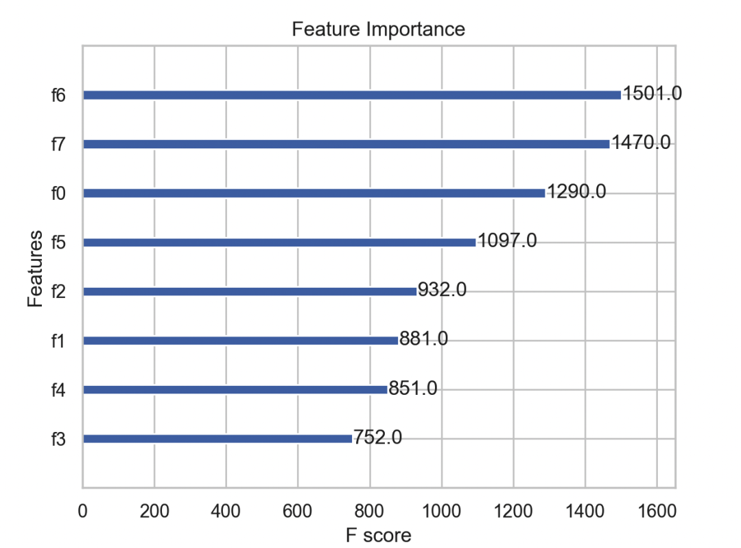
5. Visualization

Feature Importance

xgb.plot_importance(model)
plt.title('Feature Importance')
plt.show()

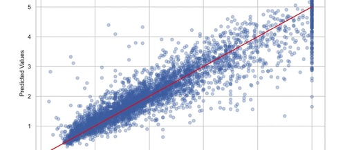
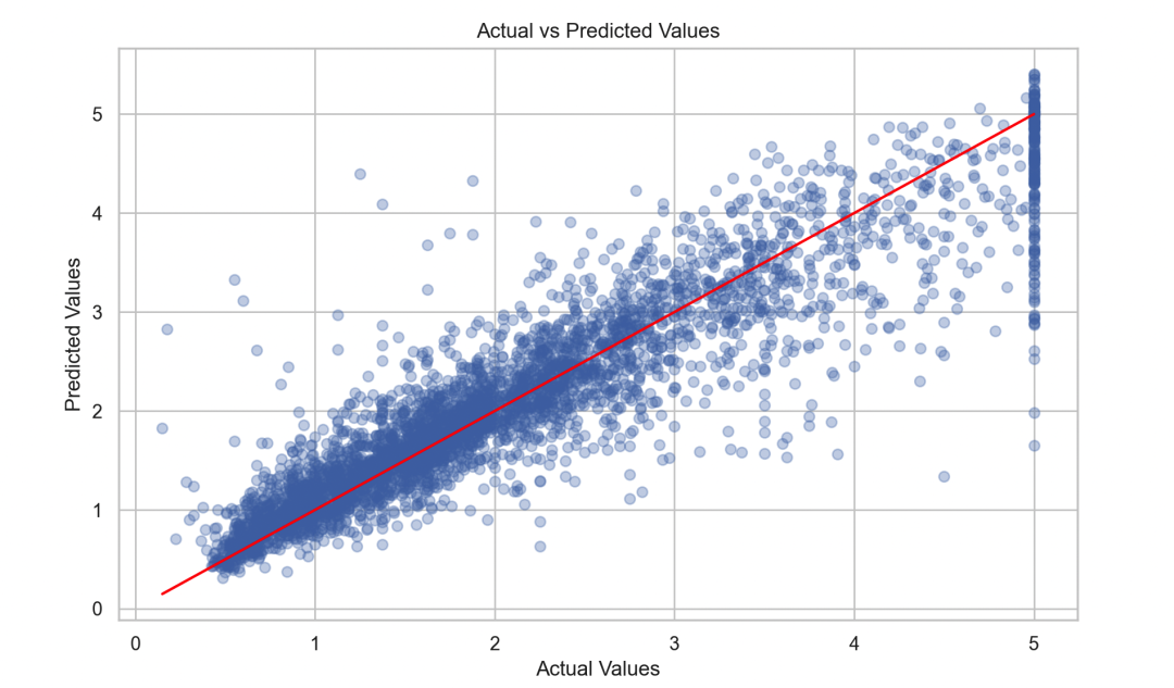
Comparison of Actual vs Predicted Values

plt.figure(figsize=(10, 6))
plt.scatter(y_test, y_pred, alpha=0.3)
plt.plot([min(y_test), max(y_test)], [min(y_test), max(y_test)], color='red')
plt.xlabel('Actual Values')
plt.ylabel('Predicted Values')
plt.title('Actual vs Predicted Values')
plt.show()

6. Algorithm Optimization

The key to optimizing XGBoost lies in fine-tuning parameters and appropriately processing data. Here are some important optimization strategies:

1. Learning Rate Adjustment: Improve model performance by reducing the learning rate and increasing the number of trees.

2. Tree Parameters: Adjust parameters like max_depth, min_child_weight to control tree complexity and prevent overfitting.

3. Regularization Parameters: Adjust lambda and alpha parameters to further control model complexity.

4. Data Sampling: Use subsample and colsample_bytree parameters to reduce the risk of overfitting.

5. Early Stopping: Monitor model performance on the validation set and use early stopping to prevent overfitting.

Below are some areas for further optimization that you can refer to~

from xgboost import early_stopping
import pandas as pd

evals = [(dtest, 'test')]

# Retrain the model with early stopping
optimized_model = xgb.train(
    params=best_params,
    dtrain=dtrain,
    num_boost_round=1000,
    evals=evals,
    early_stopping_rounds=50
)

# Predict and calculate MSE
y_pred_optimized = optimized_model.predict(dtest)
mse_optimized = mean_squared_error(y_test, y_pred_optimized)
print(f"Optimized Mean Squared Error: {mse_optimized}")

In summary, we completed a comprehensive XGBoost example from data loading, preprocessing, model training, parameter tuning to visualization. We found the best parameters through grid search and trained the model using these parameters, ultimately visualizing feature importance and model prediction results. The optimization steps shown above illustrate how to further enhance model performance.

If you have any other questions, feel free to leave a message in the comments~