Why Does XGBoost Excel in Machine Learning Competitions?

Original by Machine Heart

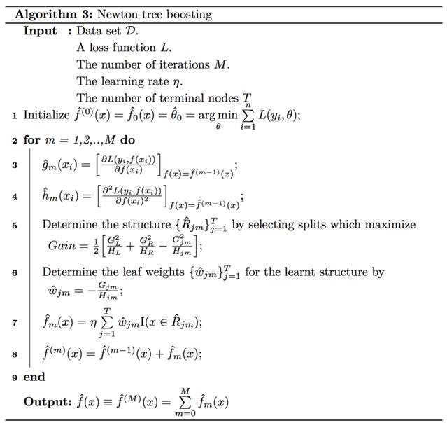
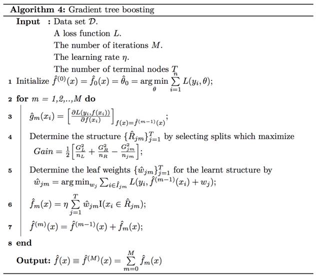
Authors: Yi Jin, Joni Chuang

Participants: Panda

Didrik Nielsen’s master’s thesis at the Norwegian University of Science and Technology, “Tree Boosting with XGBoost: Why Does XGBoost Win ‘Every’ Machine Learning Competition?” analyzes the differences between XGBoost and traditional MART and its advantages in machine learning competitions. The technical analysts at Machine Heart have interpreted this 110-page thesis, extracting its key points and core ideas into this article. The original text was published on the English official website of Machine Heart.

• Original thesis: https://brage.bibsys.no/xmlui/bitstream/handle/11250/2433761/16128_FULLTEXT.pdf

• Interpretation article in English: https://syncedreview.com/2017/10/22/tree-boosting-with-xgboost-why-does-xgboost-win-every-machine-learning-competition/

Introduction

Tree boosting has proven effective for predictive mining in classification and regression tasks.

For many years, the tree boosting algorithm chosen was MART (multiple additive regression tree). However, since 2015, a new and consistently winning algorithm has emerged: XGBoost. This algorithm re-implemented tree boosting and has achieved outstanding results in Kaggle and other data science competitions, gaining widespread popularity.

In the thesis “Tree Boosting with XGBoost – Why Does XGBoost Win ‘Every’ Machine Learning Competition?”, Didrik Nielsen from the Norwegian University of Science and Technology investigates:

1. The differences between XGBoost and traditional MART

2. The reasons why XGBoost can win “every” machine learning competition

The thesis is divided into three main parts:

1. A review of some core concepts in statistical learning

2. An introduction to boosting, explained in terms of numerical optimization in function space; further discussion of additional tree methods and core elements of tree boosting

3. A comparison of the properties of the tree boosting algorithms implemented by MART and XGBoost; an explanation of the reasons for XGBoost’s popularity

Basic Concepts of Statistical Learning

The thesis begins by introducing supervised learning tasks and discussing model selection techniques.

The goal of machine learning algorithms is to minimize the expected generalization error, also known as risk. If we knew the true distribution P(x,y), minimizing risk would be an optimization task solvable by optimization algorithms. However, we do not know the true distribution; we only have a sample set for training. We need to convert this into an optimization problem, i.e., minimizing the expected error on the training set. Therefore, the empirical distribution defined by the training set replaces the true distribution. This viewpoint can be expressed in the following statistical formula:

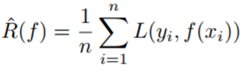
Where is the empirical estimate of the true risk R(f) of the model. L(.) is a loss function, such as the squared error loss function (commonly used in regression tasks), and other loss functions can be found here: http://www.cs.cornell.edu/courses/cs4780/2017sp/lectures/lecturenote10.html. n is the number of samples.

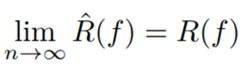
When n is sufficiently large, we have:

ERM (Empirical Risk Minimization) is an inductive principle that relies on minimizing empirical risk (Vapnik, 1999). The empirical risk minimization operation f hat is the empirical approximation of the objective function, defined as:

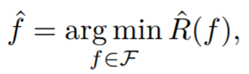
Where F belongs to a certain class of functions, known as a model class (model class), such as constants, linear methods, local regression methods (k-nearest neighbors, kernel regression), spline functions, etc. ERM is the standard for selecting the optimal function f hat from the function set F.

This model class and the ERM principle can transform the learning problem into an optimization problem. The model class can be seen as a candidate solution function, while ERM provides us with the criterion for selecting the minimization function.

There are many methods for optimization problems, among which two main methods are gradient descent and Newton’s method; MART and XGBoost use these two methods respectively.

The thesis also summarizes common learning methods:

1. Constants

2. Linear methods

3. Locally optimal methods

4. Basis function expansion: explicit nonlinear terms, splines, kernel methods, etc.

5. Adaptive basis function models: GAM (Generalized Additive Model), neural networks, tree models, boosting

Another machine learning concept is model selection, which considers different learning methods and their hyperparameters. The primary question has always been: is it better to increase the complexity of the model? The answer is always related to the model’s generalization performance. As shown in Figure 1, we may achieve better performance with a more complex model (avoiding underfitting), but we may also lose generalization performance (overfitting):

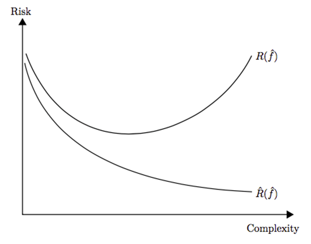
Figure 1: Generalization Performance vs Training Error

For squared loss, the classic bias-variance decomposition using expected conditional risk allows us to observe the change in risk relative to complexity:

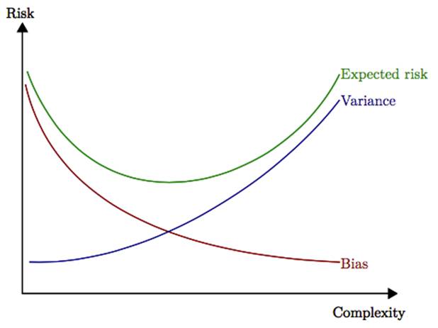
Figure 2: Expected Risk vs Variance vs Bias

A commonly used technique for this is regularization. By implicitly and explicitly considering the fit and imperfection of the data, regularization helps control the variance of the fit. It also aids the model in achieving better generalization performance.

Different model classes measure complexity in different ways. LASSO and Ridge (Tikhonov regularization) are two commonly used measurement methods in linear regression. We can directly apply constraints (subsetting, stepwise) or penalties (LASSO, Ridge) to complexity measurements.

Understanding Boosting, Tree Methods, and Tree Boosting

Boosting

Boosting is a learning algorithm that uses multiple simpler models to fit data, and these simpler models are referred to as base learners or weak learners. The learning method is to adaptively fit the data using base learners with the same or slightly different parameter settings.

Freund and Schapire (1996) introduced the first development: AdaBoost. In fact, AdaBoost minimizes the exponential loss function and iteratively trains weak learners on weighted data. Researchers have also proposed a new boosting algorithm that minimizes the second-order approximation of the log loss: LogitBoost.

Breiman (1997a,b 1998) was the first to propose that boosting algorithms could be used as numerical optimization techniques in function space. This idea allowed boosting techniques to be applied to regression problems as well. This thesis discusses two main numerical optimization methods: gradient boosting and Newton boosting (also known as second-order gradient boosting or Hessian boosting, because it uses the Hessian matrix). Now, let us understand the boosting algorithm step by step.

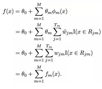
Boosting fits an ensemble model:

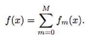
It can be written as an adaptive basis function model:

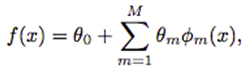
Where f_0(x)=θ_0 and f_m(x)=θ_m*Φ_m(x), m=1,…,M, and Φm are the basis functions that are sequentially accumulated to improve the fit of the current model.

Therefore, most boosting algorithms can be seen as solving the following equation accurately or approximately at each iteration:

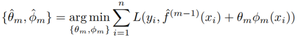
Thus, AdaBoost solves the above equation for the exponential loss function, with the constraint that: Φm is a classifier from A={-1,1}. Gradient boosting or Newton boosting approximates the above equation for any suitable loss function.

The algorithms for gradient boosting and Newton boosting are as follows:

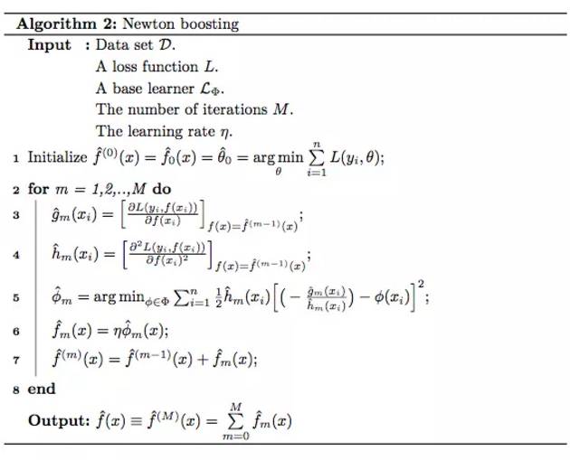
is the gradient

is the weak learner learned from the data

Gradient boosting: is the step size determined by line search

Newton boosting: is the empirical Hessian

The most commonly used base learners are regression trees (such as CART), as well as component-wise linear models or component-wise smoothing splines. The principle of base learners is to be simple, i.e., have a high bias but low variance.

The hyperparameters in boosting methods include:

1. Number of iterations M: The larger M is, the greater the possibility of overfitting, so a validation set or cross-validation set is needed.

2. Learning rate η: Reducing the learning rate often improves generalization performance, but it also increases M, as shown in the figure below.

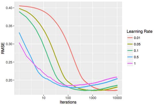
Out-of-sample RMSE for different learning rates on the Boston Housing dataset

Tree Methods

Tree models are simple and interpretable models. Their predictive ability is indeed limited, but when combined with multiple tree models (such as bagged trees, random forests, or in boosting), they can become a powerful predictive model.

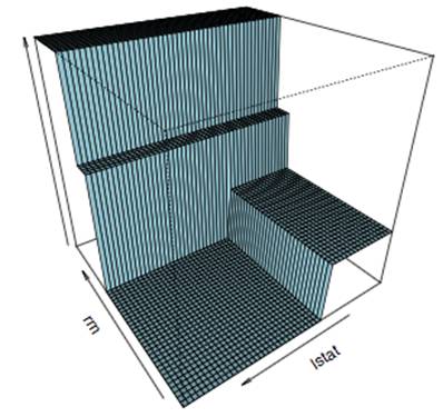
We can view tree models as dividing the feature space into several different rectangular and non-overlapping regions, and then fitting some simple models. The following figure shows the visualization results obtained using the Boston Housing data:

The number of terminal nodes and the depth of the tree can be seen as measures of the complexity of the tree model. To generalize this model, we can easily apply a complexity constraint on the complexity measure, or apply a penalty on the number of terminal nodes or leaf weights (this method is used by XGBoost).

Since learning the structure of such trees is NP-hard, learning algorithms often compute an approximate solution. There are many different learning algorithms in this regard, such as CART (Classification and Regression Trees), C4.5, and CHAID. This thesis describes CART because MART uses CART, and XGBoost also implements a tree model related to CART.

CART grows trees in a top-down manner. By considering each split parallel to the coordinate axes, CART can choose the split that minimizes the objective. In the second step, CART considers each parallel split within each region. At the end of this iteration, the best split is selected. CART repeats all these steps until a stopping criterion is reached.

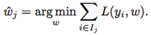
Given a region Rj, learning its weight wj is usually straightforward. Let Ij be the set of indices belonging to region Rj, i.e., xi∈Rj, where i∈Ij.

Its weight is estimated as:

For a tree model f_hat, the empirical risk is:

Where we let L_j hat represent the cumulative loss at node j. During the learning process, the current tree model is represented by f_before hat and f_after hat.

We can calculate the gain brought by the considered split:

For each split, the gain for each possible node and each possible split is calculated, and the maximum gain is taken.

Now let us consider missing values. CART uses surrogate variables to handle missing values, meaning that for each predictor, we only use non-missing data to find the split, and then based on the main split, find alternative predictors to simulate that split. For example, suppose in the given model, CART splits data based on household income. If an income value is unavailable, CART may choose education level as a good alternative.

However, XGBoost handles missing values by learning the default direction. XGBoost automatically learns the best direction when a value is missing. This can be equivalently seen as automatically “learning” the best imputation value for missing values based on the reduction in training loss.

For categorical predictors, we can handle them in two ways: grouped categories or independent categories. CART handles grouped categories, while XGBoost requires independent categories (one-hot encoding).

This thesis summarizes the advantages and disadvantages of tree models in list form:

Advantages (Hastie et al., 2009; Murphy, 2012):

• Easy to interpret

• Can be built relatively quickly

• Can naturally handle continuous and categorical data

• Can naturally handle missing data

• Robust to outliers in the input

• Invariant when input undergoes monotonic transformations

• Performs implicit variable selection

• Can capture nonlinear relationships in the data

• Can capture high-order interactions between inputs

• Scales well to large datasets

Disadvantages (Hastie et al., 2009; Kuhn and Johnson, 2013; Wei-Yin Loh, 1997; Strobl et al., 2006):

• Often selects predictors with a higher number of different values

• May overfit when predictors have many categories

• Unstable, with good variance

• Lack of smoothness

• Difficult to obtain stacked structures

• Predictive performance is often limited

Tree Boosting

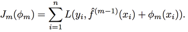
Building on the developments above, we now combine the boosting algorithm with the base learner tree methods.

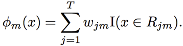
The boosted tree model can be seen as an adaptive basis function model, where the basis functions are regression trees:

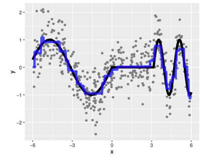
The boosted tree model (boosting tree model) is the sum of multiple trees fm, so it is also referred to as a tree ensemble or additive tree model. Therefore, it is smoother than a single tree model, as shown in the figure below:

Visualization of the additive tree model fitted on the Boston Housing data

There are many methods to implement regularization on boosted tree models:

1. Regularization on basis function expansions

2. Regularization on individual tree models

3. Randomization

Generally, boosted trees often use shallow regression trees, i.e., regression trees with only a few terminal nodes. Compared to deeper trees, such trees have lower variance but higher bias. This can be achieved by applying complexity constraints.

One of the advantages of XGBoost over MART is the penalty on complexity, which is not common for additive tree models. The penalty term in the objective function can be written as:

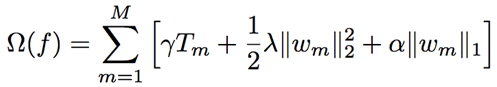
Where the first term is the number of terminal nodes for each individual tree, the second term is L2 regularization on that term’s weights, and the last term is L1 regularization on that term’s weights.

Friedman (2002) was the first to introduce randomization, which is achieved through stochastic gradient descent, including row subsampling at each iteration. Randomization helps improve generalization performance. There are two methods of subsampling: row subsampling and column subsampling. MART only includes row subsampling (without alternatives), while XGBoost includes both row and column subsampling.

As previously discussed, MART and XGBoost use two different boosting algorithms to fit additive tree models, referred to as GTB (Gradient Tree Boosting) and NTB (Newton Tree Boosting). Both algorithms aim to minimize the following at each iteration m:

Its basis function is a tree:

The general steps include three stages:

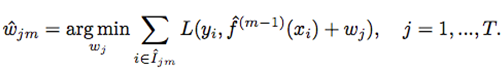
1. Determine a fixed candidate tree structure’s leaf weights;

2. Propose different tree structures using the weights determined in the previous stage, thus determining the tree structure and regions;

3. Once the tree structure is determined, the final leaf weights in each terminal node (where j=1,..,T) are also determined.

Algorithms 3 and 4 extend the algorithms 1 and 2 using trees as basis functions:

XGBoost vs MART: Differences

Finally, the thesis compares the details of the two tree boosting algorithms and attempts to provide better reasons for XGBoost.

Algorithm-Level Comparison

As discussed in previous sections, both XGBoost and MART solve the same empirical risk minimization problem through simplified FSAM (Forward Stage Additive Modelling):

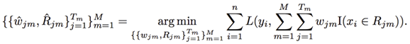
That is, without using greedy search, but adding one tree at a time. In the m-th iteration, a new tree is learned using the following:

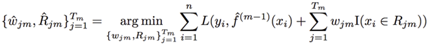
XGBoost uses the above Algorithm 3, which approximates this optimization problem using Newton Tree Boosting. MART uses the above Algorithm 4, which does this using Gradient Tree Boosting. The differences between these two methods lie first in how they learn the tree structure, and then in how they learn the leaf weights assigned to the learned tree structure.

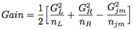
Looking at these algorithms, we can find that Newton Tree Boosting has the Hessian matrix, which plays a key role in determining the tree structure, XGBoost:

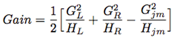
While MART using Gradient Tree Boosting is:

Then, XGBoost can directly define the leaf weights of Newton Tree Boosting as:

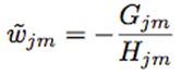
While MART defines it as:

In summary, the Hessian used by XGBoost is a higher-order approximation that can learn better tree structures. However, MART performs better in determining leaf weights, but for tree structures with lower accuracy.

In terms of the applicability of loss functions, Newton Tree Boosting requires the loss function to be twice differentiable due to the use of the Hessian matrix. Therefore, it has stricter requirements on the choice of loss functions, which must be convex.

When the Hessian is equal to 1 everywhere, these two methods are equivalent, which is the case for the squared error loss function. Therefore, if we use any loss function other than the squared error loss function, with the help of Newton Tree Boosting, XGBoost should learn tree structures better. However, Gradient Tree Boosting is more accurate in subsequent leaf weights. Thus, it cannot be compared mathematically.

Nevertheless, the authors of the thesis tested them on two standard datasets: Sonar and Ionosphere (Lichman, 2013). This empirical comparison used trees with 2 terminal nodes without other regularization, and these data also had no categorical features or missing values. Gradient Tree Boosting also added a line search, as shown by the red line in the figure.

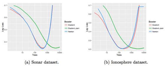
This comparison figure illustrates that both methods can be executed seamlessly. Moreover, the line search indeed enhances the convergence speed of Gradient Tree Boosting.

Regularization Comparison

Regularization parameters actually fall into three categories:

1. Boosting parameters: Number of trees M and learning rate η

2. Tree parameters: Constraints and penalties on the complexity of individual trees

3. Randomization parameters: Row subsampling and column subsampling

The main differences between the two boosting methods focus on tree parameters and randomization parameters.

For tree parameters, each tree in MART has the same number of terminal nodes, while XGBoost may also include terminal node penalties γ, so the number of terminal nodes may differ and is within the maximum number of terminal nodes. XGBoost also implements L2 regularization on leaf weights and will also implement L1 regularization on leaf weights.

In terms of randomization parameters, XGBoost provides both column subsampling and row subsampling, while MART only provides row subsampling.

Why Can XGBoost Win ‘Every’ Competition?

Using simulated data, the authors of the thesis first demonstrate that tree boosting can be seen as adaptively determining local neighborhoods.

Using

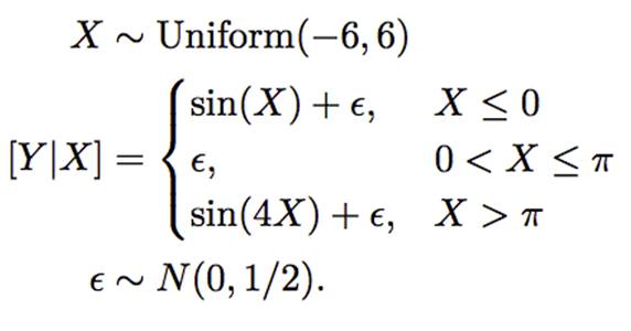
Generate

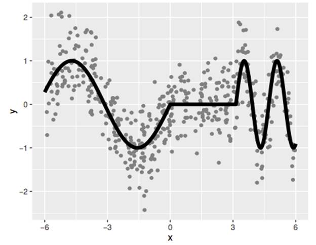
Then use local linear regression (with two different flexibilities of fitting) to fit it:

Then use smoothing spline functions (with two different flexibilities of fitting) to fit it:

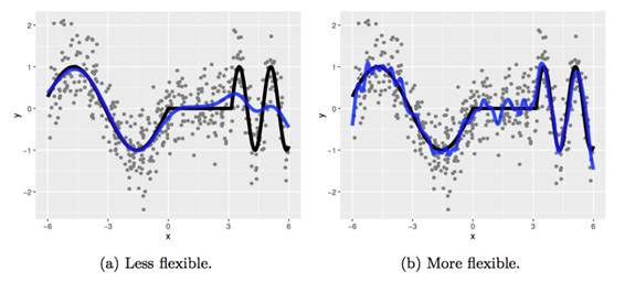
Now we try fitting a boosted tree stump (two terminal nodes):

This paper details how the weight function influences the determination of the fit and shows that tree boosting can be seen as directly considering the bias-variance trade-off during the fitting phase. This helps keep the neighborhood as large as possible to avoid unnecessary increases in variance, and only reduces it when complex structures are evident.

Although when it comes to high-dimensional problems, tree boosting “defeats” the curse of dimensionality without relying on any distance metrics. Additionally, the similarity between data points can be learned from data through adaptive adjustments of neighborhoods. This immunizes the model against the curse of dimensionality.

Moreover, deeper trees also help capture feature interactions. Therefore, there is no need to search for suitable transformations.

Thus, it is the help of boosted tree models (i.e., adaptively determining neighborhoods) that MART and XGBoost generally achieve better fits than other methods. They can perform automatic feature selection and capture high-order interactions without crashing.

By comparing MART and XGBoost, although MART does set the same number of terminal nodes for all trees, XGBoost sets Tmax and a regularization parameter that makes the trees deeper while still keeping variance low. Compared to the gradient boosting of MART, the Newton boosting used by XGBoost is likely to learn better structures. XGBoost also includes an additional randomization parameter, namely column subsampling, which helps further reduce the correlation of each tree.

Analyst’s Perspective from Machine Heart

This paper starts from the basics and then provides a detailed interpretation, which can help readers understand the algorithms behind boosting tree methods. Through empirical and simulated comparisons, we gain a better understanding of the key advantages of boosting trees compared to other models and the reasons why XGBoost outperforms typical MART. Thus, we can say that XGBoost brings a new way to improve boosting trees.

This analyst has participated in several Kaggle competitions and understands the widespread interest in XGBoost and the extensive discussions on how to tune the hyperparameters of XGBoost. I believe this article can inspire and assist beginners and intermediate competitors in better understanding XGBoost in detail.

References

• Chen, T. and Guestrin, C. (2016). Xgboost: A scalable tree boosting system. In Proceedings of the 22Nd ACM SIGKDD International Conference on Knowledge Discovery and Data Mining, KDD ’16, pages 785–794, New York, NY, USA. ACM.

• Freund, Y. and Schapire, R. E. (1996). Experiments with a new boosting algorithm. In Saitta, L., editor, Proceedings of the Thirteenth International Conference on Machine Learning (ICML 1996), pages 148–156. Morgan Kaufmann.

• Friedman, J. H. (2002). Stochastic gradient boosting. Comput. Stat. Data Anal., 38(4):367–378.

• Hastie, T., Tibshirani, R., and Friedman, J. (2009). The Elements of Statistical Learning: Data Mining, Inference, and Prediction, Second Edition. Springer Series in Statistics. Springer.

• Kuhn, M. and Johnson, K. (2013). Applied Predictive Modeling. SpringerLink: Bücher. Springer New York.

• Lichman, M. (2013). UCI machine learning repository.

• Murphy, K. P. (2012). Machine Learning: A Probabilistic Perspective. The MIT Press.

• Strobl, C., Boulesteix, A. L., and Augustin, T. (2006). Unbiased split selection for classification trees based on the Gini index. Technical report.

• Vapnik, V. N. (1999). An overview of statistical learning theory. Trans. Neur. Netw., 10(5):988–999.

• Wei-Yin Loh, Y.-S. S. (1997). Split selection methods for classification trees. Statistica Sinica, 7(4):815–840.

• Wikipedia::Lasso. https://en.wikipedia.org/wiki/Lasso_(statistics)

• Wikipedia::Tikhonov regularization. https://en.wikipedia.org/wiki/Tikhonov_regularization

Click [Read Original] to sign up for the competition. For the US region, please click the competition homepage US to enter the registration channel for the US region.