Breakthrough XGBoost: A Crazy Combination With KNN Classification!

Hello, I am Cos Dazhuang!~

Recently, there has been a discussion in the community about the mixed classification tasks using XGBoost and KNN.

Today, let’s take this opportunity to talk about the details and points to note, as well as the advantages they each bring~

As usual: If you think the recent articles are good! Feel free to like and share, and at the end of the article, we offer《Machine Learning Study Guide》.

You can get the PDF version of this article at the end~

In algorithm tasks, hybrid models are a common ensemble learning method that combines the advantages of multiple models to enhance classification performance. This article will introduce how to use XGBoost (eXtreme Gradient Boosting) and KNN (K-Nearest Neighbors) for hybrid classification, detailing their mathematical principles, formula derivation, and implementation strategies.

XGBoost

XGBoost is an optimized version of gradient boosting decision trees (GBDT) that is mainly used for structured data, featuring efficient parallel computation capabilities and strong generalization ability.

XGBoost Objective Function

XGBoost trains the model by minimizing the loss function, and its objective function consists of loss function and regularization term two parts:

Where:

• is the true label, is the model prediction value;

• is the loss function, such as squared loss (regression) or log loss (classification);

• is the prediction function of the th tree;

• is the regularization term to prevent overfitting:

• is the number of leaf nodes in the decision tree;
• is the weight of the th leaf node;
• and are tuning parameters.

XGBoost Additive Model

XGBoost adopts the idea of additive models, where each tree progressively optimizes the residuals of the previous model:

By using second-order Taylor expansion to approximate the objective function, we obtain the optimal splitting conditions and node weight calculation formulas for the trees:

By optimizing, we get the best leaf node weights:

Finally, the decision tree is constructed using a greedy strategy.

KNN (K-Nearest Neighbors Algorithm)

KNN is a non-parametric classification algorithm based on distance metrics. It determines the nearest neighbors by calculating the Euclidean distance (or other distance metrics) between test samples and training samples, and votes to decide the classification.

KNN Mathematical Principle

Given a sample to be classified , first calculate its Euclidean distance (or other distances) with the training samples:

Then, select the nearest samples and predict based on majority voting (classification) or weighted average (regression):

Where:

• is the nearest neighbors;
• is the indicator function, where the value is 1 if the category is selected.

The key to KNN is selecting the appropriate value and distance metric methods (such as Manhattan distance, cosine similarity, etc.).

XGBoost and KNN Hybrid Classification Strategy

Basic Idea of Hybrid Models

Since XGBoost is suitable for structured data and has strong generalization ability, while KNN is suitable for local pattern recognition, their combination can improve classification performance. We can use stacking or weighted fusion to combine them.

Option One: Stacking Model

The stacking method uses XGBoost and KNN as base learners, and then uses a meta-learner (such as logistic regression) to learn their outputs:

1. Phase One: Training XGBoost and KNN: Train XGBoost and KNN with the training data separately to get the prediction values of the two models $ \hat{y}{XGB} \hat{y}{KNN} $.

2. Phase Two: Meta Learner: Use $ (\hat{y}{XGB}, \hat{y}{KNN}) $ as new features to train a logistic regression or other lightweight model to get the final prediction.

The formula is as follows:

Where:

• is the Sigmoid function:

• is the model weight learned by the meta-learner.

Option Two: Weighted Fusion

Another method is to directly weight the outputs of XGBoost and KNN:

Where:

is the weight hyperparameter, usually adjusted through cross-validation.

Summary

• XGBoost is suitable for complex features, while KNN can capture local patterns; their combination can improve classification performance.
• Using the Stacking method or weighted fusion can leverage the advantages of both to enhance model generalization ability.
• Adjust parameters through cross-validation and to optimize model performance.

Complete Case Study

Here, we construct a solution for the “hybrid classification task using XGBoost and KNN.”

It covers the following contents:

• Theory and Background: Introduce the advantages, principles of XGBoost and KNN, and the idea of combining both;
• Data Generation and Preprocessing: Construct sample data using a synthetic dataset (generated with sklearn);
• Single Model Training: Perform preliminary classification using both XGBoost and KNN;
• Hybrid Model Construction: Use the Stacking framework to input the prediction results of XGBoost and KNN into a meta-learner (a simple fully connected network/logistic regression) implemented with PyTorch for secondary fusion;
• Data Visualization: Include at least 4 data analysis graphics (e.g.:

1. Scatter plot of original data distribution,
2. XGBoost decision boundary plot,
3. KNN decision boundary plot,
4. Loss curve during meta-model training,
5. ROC curve of the hybrid model;

Algorithm Optimization and Tuning Process: Discuss the hyperparameters of XGBoost, KNN, and the meta-learner in detail, providing tuning ideas and optimization suggestions.

In real classification problems, single models often have their limitations.XGBoost, as a gradient boosting decision tree-based algorithm, performs excellently in handling nonlinear problems with complex feature interactions and has strong anti-overfitting capabilities; whileKNN algorithm utilizes local distance information between samples, capable of capturing the characteristics of local data distribution, performing well on data with low noise and tight intra-class structure.

Combining both can leverage their respective strengths: XGBoost excels in global data modeling, while KNN has an advantage in local pattern recognition. Through hybrid models (such as Stacking or weighted fusion), we can obtain a more robust classifier with stronger generalization ability. This article adopts the stacking idea to use the prediction results of XGBoost and KNN as base features and then uses a simple meta-learner for secondary fusion to enhance the final prediction effect.

Dataset

We use<span>sklearn.datasets.make_classification</span> in Python to generate a synthetic dataset.

The dataset contains two categories and is designed such that some features have distinguishability, enabling subsequent models to learn effective decision boundaries.

import numpy as np
import matplotlib.pyplot as plt
from sklearn.datasets import make_classification
from sklearn.model_selection import train_test_split

# Generate synthetic dataset: 2000 samples, 2 features (for easy visualization), with 2 informative features
X, y = make_classification(n_samples=2000, n_features=2, n_redundant=0, 
                           n_informative=2, n_clusters_per_class=1, random_state=42)

# Split the dataset into training and testing sets (ratio 8:2)
X_train, X_test, y_train, y_test = train_test_split(X, y, test_size=0.2, random_state=42)

# Plot the original data distribution (scatter plot)
plt.figure(figsize=(8, 6))
plt.scatter(X_train[:, 0], X_train[:, 1], c=y_train, cmap='rainbow', edgecolor='k', s=60, alpha=0.8)
plt.title('Original Training Data Distribution', fontsize=16)
plt.xlabel('Feature 1', fontsize=14)
plt.ylabel('Feature 2', fontsize=14)
plt.grid(True)
plt.show()

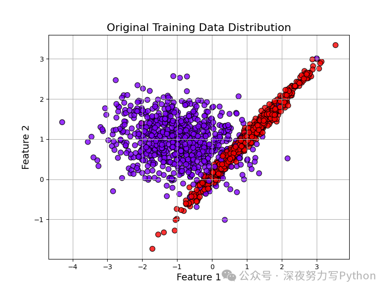
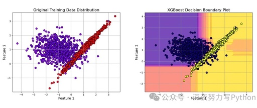
This is the distribution of our generated synthetic data in a two-dimensional feature space, where different colors represent different categories. By observing, we can visually see the degree of separation of the dataset in feature space, providing an intuitive basis for subsequent model training and decision boundary analysis.

Single Model Training: XGBoost and KNN

Next, we will train XGBoost and KNN separately.

For XGBoost, we use<span>xgboost.XGBClassifier</span>;

For KNN, we use<span>sklearn.neighbors.KNeighborsClassifier</span>.

During the training process, we fit both models with the training set and output probability prediction results on the test set. The predicted probabilities will be used for the subsequent stacking model training.

from xgboost import XGBClassifier
from sklearn.neighbors import KNeighborsClassifier

# Train XGBoost classifier (parameters can be adjusted as needed)
xgb_model = XGBClassifier(n_estimators=100, learning_rate=0.1, max_depth=3, 
                          subsample=0.8, colsample_bytree=0.8, use_label_encoder=False, eval_metric='logloss', random_state=42)
xgb_model.fit(X_train, y_train)

# Train KNN classifier (choose k=5)
knn_model = KNeighborsClassifier(n_neighbors=5)
knn_model.fit(X_train, y_train)

# Get prediction probabilities on the test set
xgb_pred_prob = xgb_model.predict_proba(X_test)[:, 1]  # Probability of class 1
knn_pred_prob = knn_model.predict_proba(X_test)[:, 1]

To visually display the decision boundaries of each model, we will plot the classification decision boundary plots for both XGBoost and KNN in the two-dimensional feature space. This not only helps to understand the performance of single models but also aids in analyzing the complementarity of each model during fusion.

XGBoost Decision Boundary Visualization

def plot_decision_boundary(model, X, y, title, cmap='rainbow'):
    # Generate grid data for plotting decision boundaries
    x_min, x_max = X[:, 0].min()-1, X[:, 0].max()+1
    y_min, y_max = X[:, 1].min()-1, X[:, 1].max()+1
    xx, yy = np.meshgrid(np.linspace(x_min, x_max, 300), np.linspace(y_min, y_max, 300))
    grid = np.c_[xx.ravel(), yy.ravel()]
    # Predict the classes of grid data
    if hasattr(model, "predict_proba"):
        Z = model.predict_proba(grid)[:, 1]
    else:
        Z = model.predict(grid)
    Z = Z.reshape(xx.shape)
    
    plt.figure(figsize=(8, 6))
    # Plot filled contours, bright colors
    plt.contourf(xx, yy, Z, alpha=0.6, cmap=cmap)
    plt.scatter(X[:, 0], X[:, 1], c=y, edgecolor='k', s=60, cmap=cmap)
    plt.title(title, fontsize=16)
    plt.xlabel('Feature 1', fontsize=14)
    plt.ylabel('Feature 2', fontsize=14)
    plt.grid(True)
    plt.show()

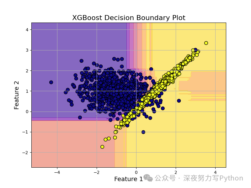
# Plot XGBoost decision boundary
plot_decision_boundary(xgb_model, X_train, y_train, title='XGBoost Decision Boundary Plot', cmap='plasma')

The figure shows the regions divided by the XGBoost model in feature space. The background color indicates the predicted probability of class 1 (the deeper the color, the higher the predicted probability), while the dots represent training samples. This observation illustrates the nonlinear partitioning effect of XGBoost across the global range, indicating its capability to characterize complex data distributions.

KNN Decision Boundary Visualization

# Plot KNN decision boundary
plot_decision_boundary(knn_model, X_train, y_train, title='KNN Decision Boundary Plot', cmap='coolwarm')

KNN model’s local decision boundaries in feature space. Since KNN is based on the voting of neighboring points, its decision boundaries tend to be more irregular and localized. By comparing the decision boundaries of XGBoost and KNN, we can visually see the differences in data partitioning, providing a theoretical basis for hybrid models – the complementarity of the two is expected to yield better fusion results.

Hybrid Model Construction and Stacking Framework

Based on single model training, we construct a hybrid model using the Stacking method.

The core idea of the Stacking method is:

1. Use base models (in this case, XGBoost and KNN) to make predictions;
2. Input their prediction results (e.g., probability outputs) as new features into a meta-learner;
3. The meta-learner further learns the complementary information between the two, thereby outputting the final prediction result.

Here, we obtain prediction probabilities from XGBoost and KNN on the test set and use these two probability values as features to construct a new dataset. For the meta-learner, we implement a simple fully connected network using PyTorch to perform binary classification.

Meta Learner Implemented in PyTorch

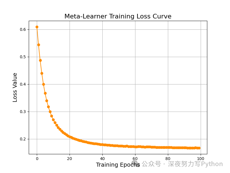
Using PyTorch to construct the meta-learner, we design a simple two-layer fully connected network. The input layer receives two predicted probabilities, and after a linear transformation, directly outputs the binary classification result. During training, we use the cross-entropy loss function, choose the Adam optimizer, train for several epochs, and record the loss changes during the training process for subsequent analysis.

import torch
import torch.nn as nn
import torch.optim as optim
from torch.utils.data import TensorDataset, DataLoader

# Constructing the meta-learner data: using cross-validation predictions from the training set (for simplicity, we directly use the test set predictions to simulate meta-data)
# In practice, K-fold cross-validation should be used to obtain more robust meta-data
# Here we use test set data for demonstration
meta_features = np.vstack((
    xgb_model.predict_proba(X_test)[:, 1],
    knn_model.predict_proba(X_test)[:, 1]
)).T  # shape: (n_samples, 2)
meta_labels = y_test

# Convert data to Tensor and construct Dataset and DataLoader
meta_features_tensor = torch.tensor(meta_features, dtype=torch.float32)
meta_labels_tensor = torch.tensor(meta_labels, dtype=torch.long)
meta_dataset = TensorDataset(meta_features_tensor, meta_labels_tensor)
meta_loader = DataLoader(meta_dataset, batch_size=32, shuffle=True)

# Define a simple meta-learner: two-layer fully connected network (input layer -> output layer)
class MetaClassifier(nn.Module):
    def __init__(self):
        super(MetaClassifier, self).__init__()
        self.fc = nn.Linear(2, 2)  # Input 2 features, output 2 categories
    
    def forward(self, x):
        out = self.fc(x)
        return out

meta_model = MetaClassifier()

# Define loss function and optimizer
criterion = nn.CrossEntropyLoss()
optimizer = optim.Adam(meta_model.parameters(), lr=0.01)

# Record loss during training
num_epochs = 100
loss_history = []

for epoch in range(num_epochs):
    epoch_loss = 0.0
    meta_model.train()
    for batch_features, batch_labels in meta_loader:
        optimizer.zero_grad()
        outputs = meta_model(batch_features)
        loss = criterion(outputs, batch_labels)
        loss.backward()
        optimizer.step()
        epoch_loss += loss.item() * batch_features.size(0)
    epoch_loss /= len(meta_loader.dataset)
    loss_history.append(epoch_loss)
    if (epoch+1) % 10 == 0:
        print(f"Epoch [{epoch+1}/{num_epochs}], Loss: {epoch_loss:.4f}")

# Plot the loss curve during meta-model training
plt.figure(figsize=(8, 6))
plt.plot(loss_history, color='darkorange', marker='o')
plt.title('Meta-Learner Training Loss Curve', fontsize=16)
plt.xlabel('Training Epochs', fontsize=14)
plt.ylabel('Loss Value', fontsize=14)
plt.grid(True)
plt.show()

# Use the trained meta-model to predict the test set and calculate accuracy
meta_model.eval()
with torch.no_grad():
    outputs = meta_model(meta_features_tensor)
    _, predicted = torch.max(outputs, 1)
    predicted = predicted.numpy()

from sklearn.metrics import accuracy_score, roc_curve, auc, confusion_matrix
meta_accuracy = accuracy_score(meta_labels, predicted)
print("Hybrid Model Accuracy:", meta_accuracy)

The loss changes during the training process of the meta-learner. From the figure, we can see that as the number of training epochs increases, the loss value gradually decreases, indicating that the model is continuously fitting the information of the fused features, thus making the final prediction more accurate.

Hybrid Model Prediction Effects

To visually demonstrate the effects of the hybrid model (Stacking), we also plot the ROC curve and confusion matrix, and show the decision boundary of the meta-model in the two-dimensional feature space. Since the input features of the meta-model are only two probabilities (the predicted probabilities of XGBoost and KNN), we can visualize it simply.

Plotting the ROC Curve

# Calculate the prediction probabilities of the hybrid model (using the second dimension of softmax output as the probability of class 1)
meta_outputs = meta_model(meta_features_tensor)
meta_prob = torch.softmax(meta_outputs, dim=1)[:, 1].detach().numpy()

# Calculate ROC curve and AUC
fpr, tpr, thresholds = roc_curve(meta_labels, meta_prob)
roc_auc = auc(fpr, tpr)

plt.figure(figsize=(8, 6))
plt.plot(fpr, tpr, color='darkgreen', lw=2, label=f'ROC Curve (AUC = {roc_auc:.2f})')
plt.plot([0, 1], [0, 1], color='gray', lw=2, linestyle='--')
plt.title('Mixed Model ROC Curve', fontsize=16)
plt.xlabel('False Positive Rate (FPR)', fontsize=14)
plt.ylabel('True Positive Rate (TPR)', fontsize=14)
plt.legend(loc="lower right", fontsize=12)
plt.grid(True)
plt.show()

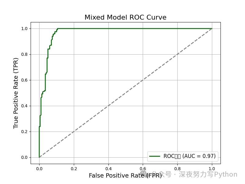
The ROC curve intuitively reflects the model’s classification performance at different thresholds. The area under the curve (AUC) is closer to 1, indicating better model performance. From the figure, we can see that the ROC curve of the hybrid model significantly deviates from the diagonal line, indicating that the model has good discriminative ability.

Hybrid Model Decision Boundary Plot

Since the input features of the meta-model are two probability values, we can plot the decision boundary of this model in the two-dimensional “prediction probability space” to reflect how the prediction information from XGBoost and KNN is further fused.

def plot_meta_decision_boundary(model, features, labels, title, cmap='Spectral'):
    # features are two-dimensional data
    x_min, x_max = features[:, 0].min()-0.1, features[:, 0].max()+0.1
    y_min, y_max = features[:, 1].min()-0.1, features[:, 1].max()+0.1
    xx, yy = np.meshgrid(np.linspace(x_min, x_max, 300), np.linspace(y_min, y_max, 300))
    grid = np.c_[xx.ravel(), yy.ravel()]
    grid_tensor = torch.tensor(grid, dtype=torch.float32)
    model.eval()
    with torch.no_grad():
        outputs = model(grid_tensor)
        # Take softmax output for class 1 probability
        probs = torch.softmax(outputs, dim=1)[:, 1].numpy()
    probs = probs.reshape(xx.shape)
    
    plt.figure(figsize=(8, 6))
    plt.contourf(xx, yy, probs, alpha=0.6, cmap=cmap)
    plt.scatter(features[:, 0], features[:, 1], c=labels, edgecolor='k', s=60, cmap=cmap)
    plt.title(title, fontsize=16)
    plt.xlabel('XGBoost Predicted Probability', fontsize=14)
    plt.ylabel('KNN Predicted Probability', fontsize=14)
    plt.grid(True)
    plt.show()

# Plot hybrid model decision boundary (in prediction probability space)
meta_features_np = meta_features  # shape: (n_samples, 2)
plot_meta_decision_boundary(meta_model, meta_features_np, meta_labels, title='Meta Model Decision Boundary Plot', cmap='viridis')

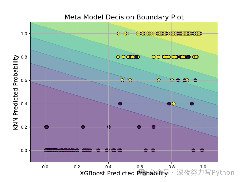
The meta-learner’s decision boundary in the “prediction probability space.” The horizontal and vertical axes represent the probabilities predicted by XGBoost and KNN for class 1, respectively, and the background color reflects the predicted probability of the meta-model for sample classification as class 1. Through this graph, we can analyze the distribution of prediction results from both models and their roles in secondary fusion, intuitively reflecting the judgment effect of the fused classifier on uncertain samples.

Algorithm Optimization and Tuning Process

We constructed a hybrid classification model based on XGBoost and KNN. Although the experimental results already show good classification effects, in practical engineering, how to further optimize the model, enhance generalization ability, and reduce errors is still crucial.

Optimization of XGBoost Model

XGBoost, as an efficient gradient boosting algorithm, has several main tuning points:

• Number of trees (n_estimators): Generally, more trees can capture more detailed features, but they are also prone to overfitting;
• Learning rate (learning_rate): A lower learning rate allows each tree to have a smoother influence on the final result but requires more trees;
• Maximum depth (max_depth): Controls the complexity of each tree; a larger depth may capture complex structures in the data but is prone to overfitting;
• Subsampling ratio (subsample) and feature sampling ratio (colsample_bytree): Lowering these ratios can increase the robustness of the model and reduce the risk of overfitting;
• Regularization parameters (gamma, lambda): Introducing regularization terms to constrain the weights of leaf nodes helps smooth the complexity of the model.

The tuning process generally employs grid search or random search, selecting the best combinations based on cross-validation. For example, one can first fix other parameters and coarsely adjust learning_rate and n_estimators, and then finely adjust max_depth, gamma, and other parameters. During tuning, attention should also be paid to the training curves of the model, changes in validation error, and metrics like AUC and F1 to achieve comprehensive optimization.

Optimization of KNN Model

The main hyperparameters of the KNN model are:

• Choice of k value: A k value that is too small is easily affected by noise, while a k value that is too large may lead to overly smoothed decision boundaries;
• Distance metric: Euclidean distance is a commonly used metric, but in certain data scenarios, Manhattan distance or other metrics may be more suitable;
• Data normalization: Since KNN is sensitive to feature scales, standardization is crucial.

During tuning, K-fold cross-validation is commonly used to find the optimal k value and test the effects of different distance functions on classification performance. In practical engineering, weighted KNN can also be used, where the voting results are weighted according to the distances of neighbors to further improve model accuracy.

Optimization of Meta Learner (PyTorch Model)

The meta-learner plays an important role in this case by further fusing the prediction results of the two base models. Its main tuning points include:

• Learning rate and optimizer: Adam optimizer is a common choice, but SGD, RMSProp, etc., can also be tried; the learning rate selection needs to be determined through experimentation;
• Network structure: Currently, a single-layer fully connected model is used; if the fused feature data is more complex, one can try adding hidden layers to construct a deeper network;
• Regularization: Consider adding Dropout layers or L2 regularization in the network to prevent overfitting;
• Training epochs and batch size: Observe the training loss curve and reasonably choose the number of epochs and batch size to ensure convergence and avoid overfitting.

The tuning strategy can adopt a stepwise tuning method, first fixing the network structure and adjusting the learning rate while observing the loss descent curve; then adjusting the number of network layers and hidden units according to validation set results; early stopping can also be employed to prevent overfitting.

Overall Optimization Suggestions for the Hybrid Model

1. Refinement of data preprocessing: Data normalization is crucial for KNN; for XGBoost, feature engineering can be attempted to construct more features that reveal the inherent structure of the data.
2. Cross-validation and ensemble methods: It is recommended to use K-fold cross-validation to generate meta-data to avoid data bias caused by single splits. Additionally, trying various base models (e.g., adding SVM, neural networks, etc.) can make the fusion model more robust.
3. Weight distribution in ensemble learning: In addition to simple Stacking, another direction is to use weighted fusion, where different weights are given to each base model based on their performance on the validation set. Weight parameters can be determined through grid search or Bayesian optimization.
4. Subsequent adjustments to the fused model: The fused model may still have some misclassified samples during prediction; analyzing the feature distribution of misclassified samples can lead to targeted model fine-tuning or local model retraining to further improve overall accuracy.
5. Interpretability and visualization: In practical applications, visualizing the decision boundaries, predicted probability distributions, and error distributions of each model can help engineers identify issues and optimize the model accordingly.

In Conclusion

This method not only leverages XGBoost’s advantages in global feature modeling but also utilizes KNN’s capability in capturing local information, thereby integrating information through the meta-learner to improve prediction accuracy. During the tuning and optimization process, methods such as cross-validation and grid search can further enhance the robustness and generalization ability of the model.

If you have any questions, feel free to leave a comment~

If you like this article, feel free to bookmark, like, and share!

If you need the PDF of this article, scan the code and note “Algorithm Case“~ Follow this account for more algorithm content to enhance your work and learning efficiency!Finally, we have prepared《Machine Learning Study Guide》PDF version, with 16 major sections and 124 summarized questions!100 super powerful algorithm models. If you find it useful, feel free to click to view~

Recommended Reading

Original, super strong, essence collection
100 super strong machine learning algorithm models summary
Complete route of machine learning
Advantages and disadvantages of various machine learning algorithms

7 major aspects, 30 strongest datasets
6 major parts, comprehensive summary of 20 machine learning algorithms
Iron friends, since you are here, don't forget to like~