Approximately 3200 words, recommended reading time 5 minutes
This article introduces the mathematical principles behind neural networks.
git clone https://github.com/omar-florez/scratch_mlp/python scratch_mlp/scratch_mlp.py
Although the technology has intuitive and modular characteristics, it is responsible for updating the trainable parameters, which has always been a topic that has not been deeply explained. Let’s use Lego blocks as a metaphor, adding one piece at a time, to build a neural network from scratch to explore its internal functions.
A Neural Network Is Like Being Made of Lego Blocks
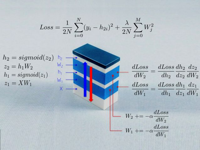
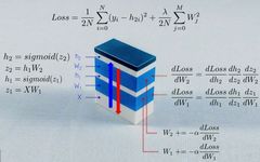
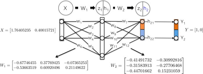
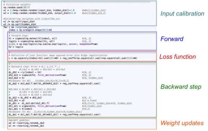
The above image describes some of the mathematical processes used when training a neural network. We will explain this in the article. One interesting point for readers is that a neural network is a stack of many modules with different objectives.
-
The input variable X feeds raw data into the neural network, which is stored in a matrix where the rows are observations and the columns are dimensions.
-
Weight W_1 maps input X to the first hidden layer h_1. Then, weight W_1 acts as a linear kernel.
-
The Sigmoid function prevents numbers in the hidden layer from falling outside the range of 0-1. The result is an array of neural activations, h_1 = Sigmoid(WX).
Why Should I Read This Article?
If you understand the internal components of a neural network, you can quickly know where to make changes when encountering problems and can devise strategies to test the invariants and expected behaviors of the algorithm you are familiar with.
Debugging machine learning models is a complex task. Experience shows that mathematical models do not work on the first try. They may yield low accuracy on new data, take a long time to train, or consume too much memory, returning large negative values or NAN predictions… In some cases, understanding how the algorithm works can make our tasks easier:
-
If training takes too long, increasing the minibatch size may be a good idea, as it can reduce the variance of observations, helping the algorithm to converge.
-
If you see NAN predictions, the algorithm may have received large gradients, causing a memory overflow. This can be seen as matrix multiplication that explodes after many iterations. Reducing the learning rate can shrink these values. Reducing the number of layers can decrease the amount of multiplication. Gradient clipping can also significantly control this issue.
-
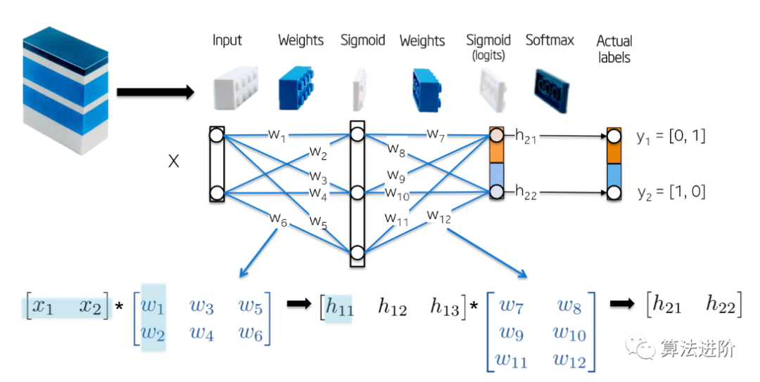
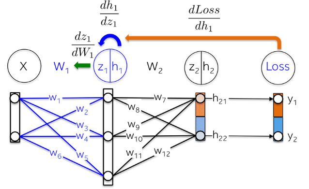
The input variable X is a two-dimensional vector. -
Weight W_1 is a 2×3 matrix with randomly initialized values. -
The hidden layer h_1 contains 3 neurons. Each neuron receives the weighted sum of observations as input, which is the inner product highlighted in green in the following image: z_1 = [x_1, x_2][w_1, w_2]. -
Weight W_2 is a 3×2 matrix with randomly initialized values. -
The output layer h_2 contains two neurons because the output of the XOR function is either 0 (y_1=[0,1]) or 1 (y_2 = [1,0]).
Network Initialization
Let’s initialize the network weights with random numbers.
Forward Step:
The goal of this step is to pass the input variable X forward through each layer of the network until we compute the vector of the output layer h_2.
This is the computation process that occurs:
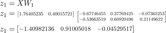
Perform a linear transformation on the input data X using weight W_1 as a linear kernel:
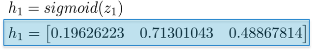
Scale the weighted sum using the Sigmoid activation function to obtain the value of the first hidden layer h_1. Note that the original 2D vector is now mapped to 3D space.
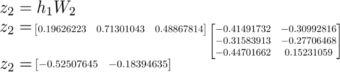
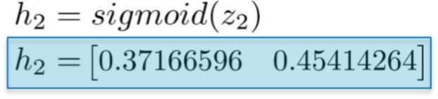
A similar process occurs in layer h_2. Let’s first calculate the weighted sum z_2 of the first hidden layer, which is now the input data.
Then compute their Sigmoid activation function. The vector [0.37166596 0.45414264] represents the log probabilities or prediction vector calculated by the network for the given input X.
Calculate Overall Loss
Also known as “actual value minus predicted value”, the goal of this loss function is to quantify the distance between the prediction vector h_2 and the artificial label y.
Note that this loss function includes a regularization term that penalizes large weights in the form of ridge regression. In other words, weights with large squared values will increase the loss function, which is the metric we want to minimize.

Backward Step:
The goal of this step is to update the weights of the neural network in the direction of minimizing the loss function. As we will see, this is a recursive algorithm that can reuse previously computed gradients and heavily relies on differential functions. Because these updates reduce the loss function, a neural network “learns” to approximate the labels of observations with known categories. This is a property known as generalization.
Unlike the forward step, this step proceeds in reverse order. It first calculates the partial derivative of the loss function with respect to each weight in the output layer (dLoss/dW_2), and then calculates the partial derivative for the hidden layer (dLoss/dW_1). Let’s explain each derivative in detail.
dLoss/dW_2:
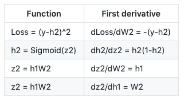
The chain rule indicates that we can break down the gradient computation of a neural network into several differential parts:

To help memorize, the table below lists some function definitions used above and their first derivatives:
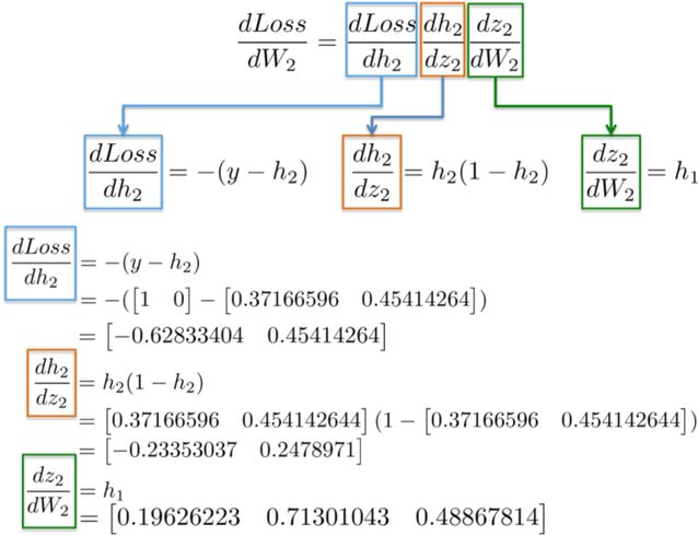
More intuitively, we want to update weight W_2 (the blue part) in the following image. To do this, we need to compute three partial derivatives along the derivative chain.

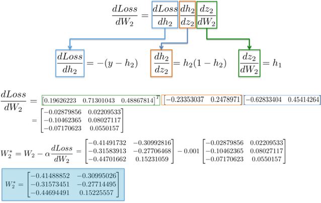
By substituting values into these partial derivatives, we can compute the derivative of W_2 as follows:
The result is a 3×2 matrix dLoss/dW_2, which will update the values of W_2 in the direction of minimizing the loss function.
dLoss/dW_1:
Calculating the chain rule used to update the weights of the first hidden layer W_1 demonstrates the possibility of reusing already computed results.
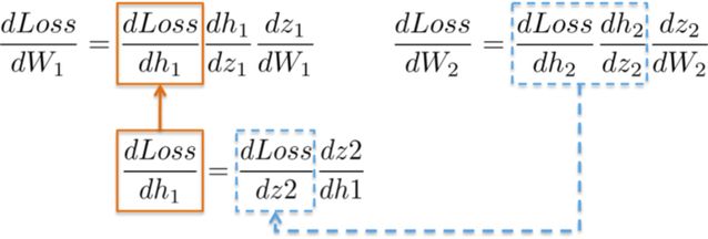
More intuitively, the path from the output layer to weight W_1 will encounter already computed partial derivatives from the later layers.
For example, the partial derivatives dLoss/dh_2 and dh_2/dz_2 have already been computed as dependencies for the output layer dLoss/dW_2 learning weights.
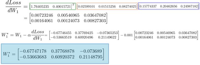
By putting all the derivatives together, we can once again perform the chain rule to update the weights of W_1 in the hidden layer.

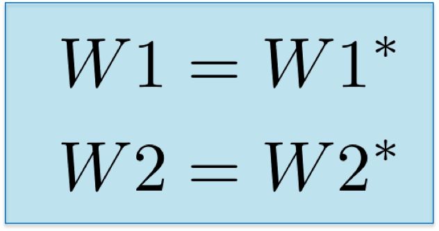
Finally, we assign new values to the weights, completing one step of training for the neural network.
Implementation
Let’s use only numpy as a linear algebra engine to convert the above mathematical equations into code. The neural network is trained in a loop, where each iteration shows the standard input data to the neural network.
In this small example, we only consider the entire dataset in each iteration. The calculations of the forward step, loss function, and backward step will yield better generalization because we update the trainable parameters with their corresponding gradients (matrices dL_dw1 and dL_dw2) in each loop.
The code is stored in this repo: https://github.com/omar-florez/scratch_mlp
Let’s run this code!
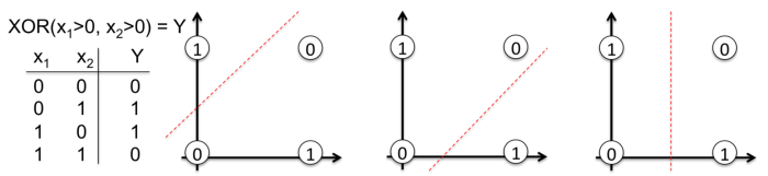
Below are some neural networks trained through many iterations that can approximate the XOR function.
Left image: Accuracy; middle image: learned decision boundary; right image: loss function.
First, let’s take a look at why the neural network with 3 neurons in the hidden layer has limited capability. This model learned to classify using a simple decision boundary, which started as a straight line but later exhibited non-linear behavior. As training continued, the loss function in the right image also significantly decreased.
The neural network with 50 neurons in the hidden layer clearly increased the model’s ability to learn complex decision boundaries. This not only yielded more accurate results but also caused gradient explosion, a significant issue when training neural networks. When gradients are very large, the multiplications in backpropagation can lead to substantial weight updates. This is why the loss function suddenly increased during the last few training steps (step > 90). The regularization term of the loss function computed the square values of weights that had become very large (sum(W²)/2N).
As you can see, this problem can be avoided by reducing the learning rate. It can be achieved by implementing a strategy that decreases the learning rate over time or by enforcing a stronger regularization, possibly L1 or L2. Gradient vanishing and gradient explosion are fascinating phenomena that we will analyze in detail later.