1. What is Deep Learning?
Deep learning (DL) is a new research direction in the field of machine learning (ML). Deep learning involves learning the inherent laws and hierarchical representations of sample data, and the information obtained during this learning process greatly aids in interpreting data such as text, images, and sound. Its ultimate goal is to enable machines to analyze and learn like humans, allowing them to recognize data such as text, images, and sound. Deep learning is a complex machine learning algorithm that has achieved results in speech and image recognition far exceeding previous related technologies.

2. The Concept of Deep Learning
Suppose we have a system S, which has n layers (S1,…Sn), with input I and output O, represented as: I => S1 => S2 => ….. => Sn => O. If the output O equals the input I, it means that the input I has undergone changes through this system without any loss of information and remains unchanged. This indicates that there has been no loss of information at any layer Si, meaning at any layer Si, it is another representation of the original information (i.e., input I). We need to automatically learn features; suppose we have a set of inputs I (such as a set of images or text), and we have designed a system S (with n layers) to adjust the parameters within the system so that its output remains the same as input I. Then we can automatically obtain a series of hierarchical features of input I, namely S1, …, Sn.
For deep learning, the idea is to stack multiple layers, meaning the output of one layer is used as the input for the next layer. Through this method, hierarchical representation of the input information can be achieved. Furthermore, the previous assumption that the output strictly equals the input is too strict; we can relax this constraint slightly, for example, we only need to ensure that the difference between input and output is minimized.
3. Deep Learning and Neural Networks
Deep learning is a new field of research in machine learning, motivated by the desire to establish and simulate neural networks that analyze and learn like the human brain. It mimics the mechanisms of the human brain to interpret data, such as images, sounds, and text. Deep learning is a type of unsupervised learning. The concept of deep learning originates from the study of artificial neural networks. A multilayer perceptron with multiple hidden layers is a type of deep learning structure. Deep learning combines low-level features to form more abstract high-level representations of attribute categories or features, to discover the distributed feature representations of data.
Deep learning itself can be considered a branch of machine learning, which can be simply understood as the evolution of neural networks. About two to three decades ago, neural networks were a particularly hot direction in the field of machine learning, but gradually faded away due to several reasons:
1) The BP algorithm, as a typical algorithm for training multilayer networks, actually consists of only a few layers, and this training method is not ideal. The local minima that commonly exist in the non-convex objective cost function of deep structures (involving multiple layers of nonlinear processing units) are the main source of training difficulty.
2) For a deep network (more than 7 layers), the residual gradient that propagates back to the earlier layers becomes too small, leading to what is known as gradient diffusion.
3) Generally, we can only use labeled data to train: however, most data is unlabeled, while the brain can learn from unlabeled data.
Deep learning and traditional neural networks have many similarities and differences.
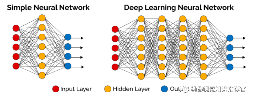
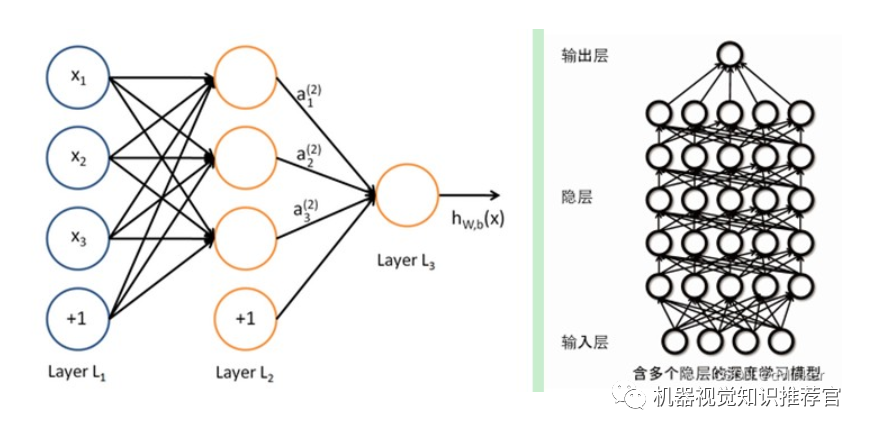
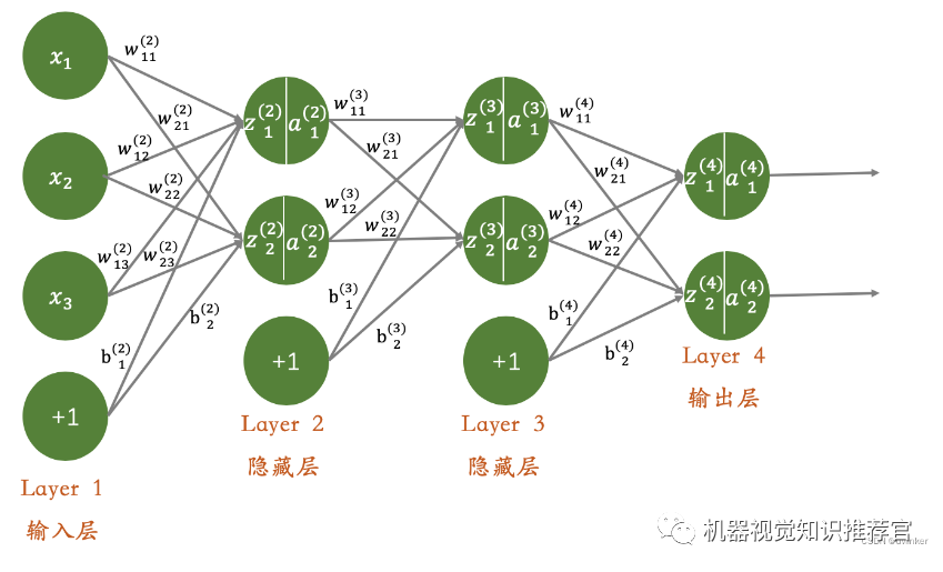
The similarity lies in that deep learning adopts a similar layered structure to neural networks, consisting of a multilayer network with an input layer, hidden layers (multiple), and an output layer, where only adjacent layers are connected, and there are no connections between nodes in the same layer or across layers. Each layer can be regarded as a logistic regression model; this layered structure is relatively close to the structure of the human brain.
To overcome the problems in training neural networks, deep learning employs a training mechanism that is quite different from neural networks. In 2006, Hinton proposed an effective method for establishing multilayer neural networks on unsupervised data. In simple terms, this is divided into two steps: first, train one layer of the network at a time, and second, fine-tune it so that the high-level representation r generated from the original representation x and the low-level representation x’ generated from the high-level representation r are as consistent as possible. The method is:
2) Once all layers are trained, Hinton uses the wake-sleep algorithm for fine-tuning.
He makes the weights between all layers except the top layer bidirectional, so the top layer remains a single-layer neural network, while the other layers become graphical models. The upward weights are used for “cognition,” and the downward weights are used for “generation.” Then, the Wake-Sleep algorithm adjusts all weights. This ensures that cognition and generation are consistent, meaning that the generated top-level representation can accurately reconstruct the bottom layer nodes as much as possible. For example, if a node at the top layer represents a face, all images of faces should activate this node, and the image generated from this result should represent a rough face image. The Wake-Sleep algorithm consists of two parts:
2) Sleep phase: The generative process generates the bottom layer’s state through the top layer’s representation (concept learned while awake) and downward weights, while modifying the upward weights between layers. This means, “If the scene in my dream does not match the corresponding concept in my mind, change my cognitive weights so that this scene appears to me as that concept.”
4. The Training Process of Deep Learning
The training process of deep learning consists of the following two steps.
4.1. First, use bottom-up unsupervised learning (i.e., starting from the bottom layer and training layer by layer to the top layer)
Using unlabeled data (labeled data can also be used) to train the parameters of each layer in a hierarchical manner. This step can be considered an unsupervised training process, which is the most significant difference from traditional neural networks (this process can be seen as a feature learning process). Specifically, first train the first layer using unlabeled data, learning the parameters of the first layer (this layer can be seen as obtaining a hidden layer of a three-layer neural network that minimizes the difference between output and input). Due to model capacity constraints and sparsity constraints, the resulting model can learn the structure of the data itself, thus obtaining features that have greater representational capacity than the input; after learning the n-1 layer, the output of the n-1 layer is used as the input for the n layer, training the n layer, thereby obtaining the parameters of each layer.
4.2. Then, top-down supervised learning (i.e., training with labeled data, propagating errors downward, and fine-tuning the network)
Based on the parameters obtained in the first step, further fine-tune the parameters of the entire multilayer model through supervised training; the first step is similar to the random initialization process of neural networks. However, since the first step of DL is not random initialization but is obtained by learning the structure of the input data, this initial value is closer to the global optimum, thus achieving better results; therefore, the effectiveness of deep learning largely depends on the feature learning process in the first step.
5. Convolutional Neural Networks
Convolutional neural networks are a type of artificial neural network and have become a research hotspot in the fields of speech analysis and image recognition. Its weight-sharing network structure makes it more similar to biological neural networks, reducing the complexity of the network model and the number of weights. This advantage is particularly evident when the input to the network is multi-dimensional images, allowing images to be directly input into the network, avoiding the complex feature extraction and data reconstruction processes in traditional recognition algorithms. Convolutional networks are a multilayer perceptron specifically designed to recognize two-dimensional shapes, and this network structure is highly invariant to translation, scaling, skewing, or other forms of deformation.
CNNs are influenced by early time-delay neural networks (TDNNs). Time-delay neural networks reduce learning complexity by sharing weights over the time dimension, making them suitable for processing speech and time-series signals.
CNNs are the first truly successful learning algorithm for training multilayer network structures. It reduces the number of parameters that need to be learned by utilizing spatial relationships to improve the training performance of the general forward BP algorithm. CNNs were proposed as a deep learning architecture to minimize the preprocessing requirements of data. In CNNs, a small portion of the image (local receptive field) serves as the input for the lowest layer of the hierarchical structure, and the information is sequentially transmitted to different layers, with each layer using a numerical filter to obtain the most significant features of the observed data. This method can capture significant features of observed data that are invariant to translation, scaling, and rotation because the local receptive fields of images allow neurons or processing units to access the most basic features, such as oriented edges or corners.
5.1. The History of Convolutional Neural Networks
In 1962, Hubel and Wiesel proposed the concept of receptive fields through their study of the visual cortex cells of cats. In 1984, Japanese scholar Fukushima proposed the neocognitron based on the concept of receptive fields, which can be seen as the first implementation of convolutional neural networks and the first application of the receptive field concept in the field of artificial neural networks. The neocognitron decomposes a visual pattern into many sub-patterns (features), which are then processed in a hierarchical and interconnected feature plane. It attempts to model the visual system so that recognition can be performed even when objects are displaced or slightly deformed.
Typically, the neocognitron contains two types of neurons: S-units responsible for feature extraction and C-units responsible for deformation resistance. The S-units involve two important parameters: the receptive field and the threshold parameter, where the former determines the number of input connections and the latter controls the response degree to the feature sub-patterns. Many scholars have been dedicated to improving the performance of the neocognitron: in traditional neocognitron, the amount of visual blur caused by C-units in the receptive field of each S-unit follows a normal distribution. If the blur effect generated at the edge of the receptive field is greater than that at the center, the S-unit will accept this non-normal blur, resulting in greater deformation tolerance. We hope to achieve a situation where the differences between the effects produced at the edges and the center of the receptive field become increasingly pronounced. To effectively form this non-normal blur, Fukushima proposed an improved neocognitron with dual C-unit layers.
Van Ooyen and Niehuis introduced a new parameter to enhance the distinguishability of the neocognitron. In fact, this parameter acts as an inhibitory signal, suppressing the excitation of neurons to repeated stimulus features. Most neural networks memorize training information in weights. According to Hebb’s learning rule, the more frequently a certain feature is trained, the easier it is to detect during subsequent recognition processes. Some scholars have also combined evolutionary computation theory with the neocognitron to weaken the training learning of repetitive stimulus features, allowing the network to focus on different features to enhance its distinguishing ability. The above describes the development process of the neocognitron, and convolutional neural networks can be seen as an extension of the neocognitron, with the neocognitron being a special case of convolutional neural networks.
5.2. The Network Structure of Convolutional Neural Networks
Convolutional neural networks are a multilayer neural network, where each layer consists of multiple two-dimensional planes, and each plane is composed of multiple independent neurons.
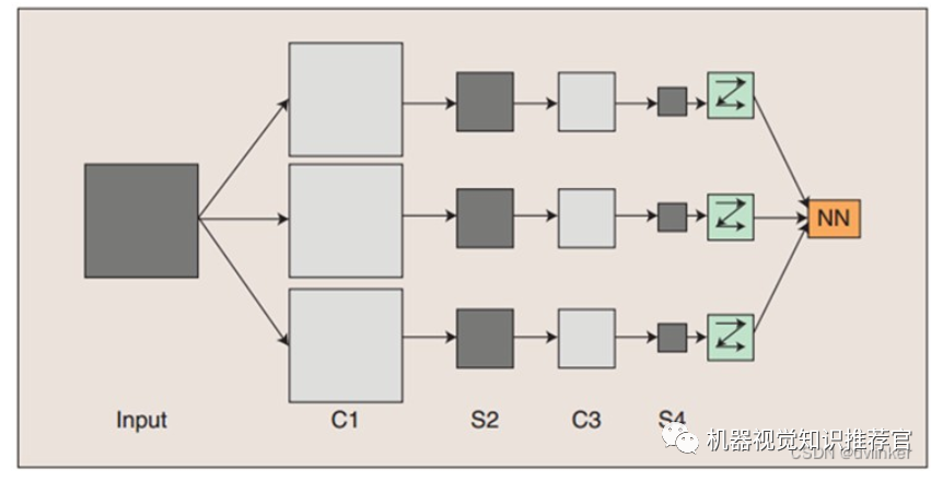
The conceptual demonstration of convolutional neural networks is shown in the figure above. The input image is convolved with three trainable filters and an additive bias, as illustrated in the first figure. After convolution, three feature maps are generated in the C1 layer, and then the four pixels in each group of feature maps are summed, weighted, and biased, producing three feature maps in the S2 layer through a Sigmoid function. These maps are then filtered to obtain the C3 layer. This hierarchical structure generates S4, similar to S2. Finally, these pixel values are rasterized and connected into a vector input to a traditional neural network to produce output.
Generally, the C layer serves as the feature extraction layer, where each neuron’s input is connected to the local receptive field of the previous layer, extracting the features of that locality. Once the local feature is extracted, its positional relationship with other features is also determined; the S layer is the feature mapping layer, where each computational layer of the network consists of multiple feature maps, and each feature map is a plane with equal weights for all neurons. The feature mapping structure employs a small influence function kernel Sigmoid function as the activation function of the convolutional network, ensuring that the feature mapping exhibits translational invariance.
Additionally, since the neurons on a mapping plane share weights, the number of free parameters in the network is reduced, simplifying the complexity of parameter selection in the network. Each feature extraction layer (C-layer) in the convolutional neural network is immediately followed by a computational layer (S-layer) for local averaging and secondary extraction. This unique two-step feature extraction structure endows the network with high distortion tolerance when recognizing input samples.
5.3. About Parameter Reduction and Weight Sharing
As mentioned earlier, one impressive aspect of CNNs is that they reduce the number of parameters that need to be trained in the neural network through receptive fields and weight sharing. But what exactly does this mean?
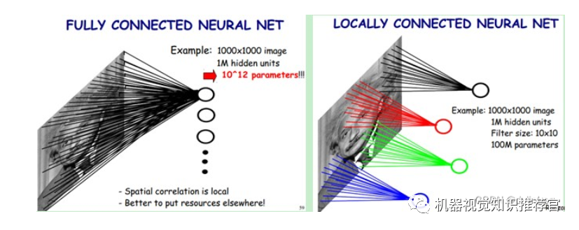
In the left figure below: if we have a 1000×1000 pixel image and 1 million hidden-layer neurons, if they are fully connected (each hidden-layer neuron connects to every pixel of the image), there would be 1000x1000x1000000=10^12 connections, which means 10^12 weight parameters. However, the spatial relationships of images are local, just as humans perceive external images through a local receptive field. Each neuron does not need to perceive the entire global image; it only needs to sense a local area of the image, and then at higher layers, these neurons that sense different local areas can combine to obtain global information. Thus, we can reduce the number of connections, which reduces the number of weight parameters that the neural network needs to train. In the right figure below: if the local receptive field is 10×10, then each hidden-layer neuron only needs to connect to this 10×10 local image, so 1 million hidden-layer neurons would only have 100 million connections, or 10^8 parameters. This reduces the number by four zeros (an order of magnitude), making training less laborious. However, it still seems like a lot; is there any other way?
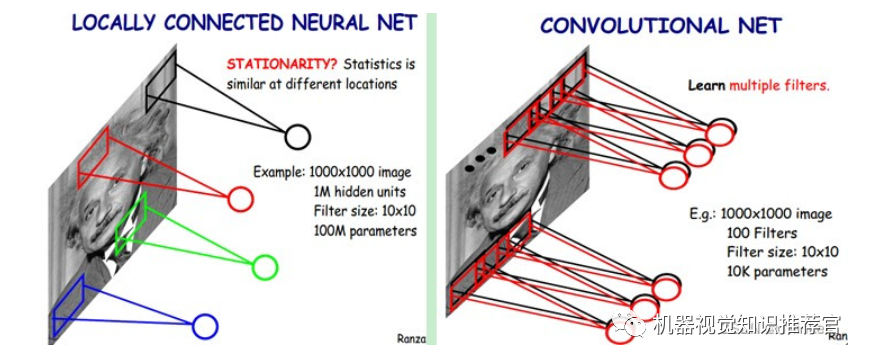
We know that each neuron in the hidden layer connects to 10×10 image regions, meaning each neuron has 10×10=100 connection weight parameters. What if we make these 100 parameters the same for each neuron? In other words, if each neuron uses the same convolution kernel to convolve the image, how many parameters do we have? Only 100 parameters! Regardless of how many neurons are in the hidden layer, there are only 100 parameters for the connections between the two layers! This is weight sharing.
If one filter, i.e., one convolution kernel, extracts a feature from the image, such as an edge in a certain direction, how do we extract different features? Just add more filters! Exactly. So suppose we add 100 different filters, each with different parameters, representing different features extracted from the input image, such as different edges. Thus, convolving the image with each filter yields different feature representations, which we call feature maps. Therefore, 100 convolution kernels yield 100 feature maps. These 100 feature maps form a layer of neurons. How many parameters are there in this layer? 100 types of convolution kernels x each convolution kernel shares 100 parameters = 100×100 = 10K, or 10,000 parameters. The different colors in the figure below represent different filters.
As mentioned earlier, the number of parameters in the hidden layer is independent of the number of neurons in the hidden layer and is only related to the size of the filter and the number of filter types. So how do we determine the number of neurons in the hidden layer? It is related to the size of the original image (i.e., the number of neurons), the size of the filter, and the sliding step of the filter in the image! For example, if my image is 1000×1000 pixels and the filter size is 10×10, assuming there is no overlap in the filter (i.e., the step size is 10), then the number of neurons in the hidden layer would be (1000×1000)/(10×10)=100×100 neurons. Note that this is just the number of neurons for one filter, i.e., one feature map. If there are 100 feature maps, it would be 100 times that. Thus, it can be seen that the larger the image, the greater the gap between the number of neurons and the number of weight parameters that need to be trained.
It is important to note that the above discussion does not consider the bias part of each neuron. Therefore, the number of weights needs to add 1. This is also shared by the same type of filter.
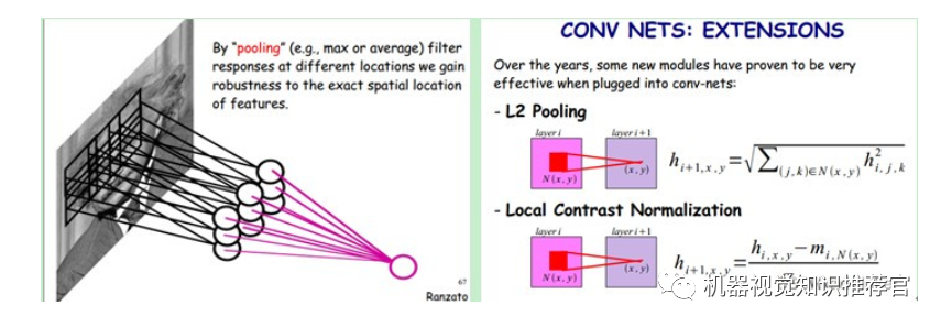
In summary, the core idea of convolutional networks is to combine local receptive fields, weight sharing (or weight replication), and temporal or spatial subsampling to achieve a certain degree of invariance to translation, scale, and deformation.
5.4. A Typical Example for Explanation
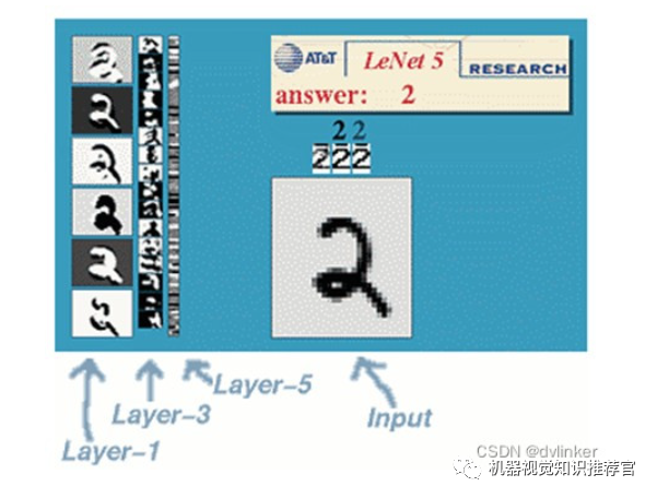
A typical convolutional network used for digit recognition is LeNet-5. Most banks in the United States used it to recognize handwritten digits on checks. Given its commercial viability, its accuracy is undeniable. After all, the combination of academia and industry is the most controversial.
Now, let’s also use this example for illustration.
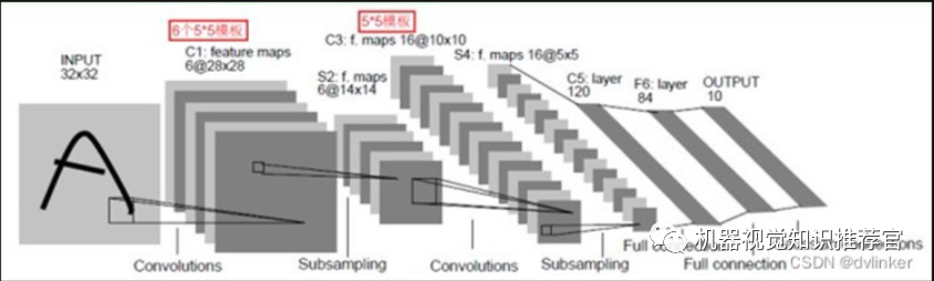
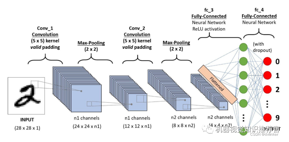
LeNet-5 has a total of 7 layers, excluding the input, and each layer contains trainable parameters (connection weights). The input image is 32*32 in size, which is larger than the largest character in the Mnist database (a recognized handwritten database). The reason for this is that it is hoped that potential obvious features such as stroke breaks or corners can appear at the center of the highest layer’s feature monitoring receptive field.
We must clarify one point: each layer has multiple feature maps, each feature map extracts one feature from the input through a convolution filter, and each feature map has multiple neurons.
The C1 layer is a convolutional layer (why convolution? A key characteristic of convolution operations is that they can enhance the original signal’s features while reducing noise), consisting of 6 feature maps. Each neuron in the feature map is connected to a 5*5 neighborhood in the input. The size of the feature map is 28*28, which prevents the connections of the input from falling outside the boundary (to avoid gradient loss during BP feedback, personal insight). C1 has 156 trainable parameters (each filter has 5*5=25 unit parameters and one bias parameter, totaling 6 filters, hence (5*5+1)*6=156 parameters), resulting in 156*(28*28)=122,304 connections.
The S2 layer is a subsampling layer (why subsampling? Utilizing the principle of local correlation in images, subsampling can reduce data processing while retaining useful information), consisting of 6 feature maps of size 14*14. Each unit in the feature map is connected to the corresponding feature map’s 2*2 neighborhood in C1. Each unit in the S2 layer sums 4 inputs, multiplies by a trainable parameter, adds a trainable bias, and the result is computed through the sigmoid function. The trainable coefficients and biases control the non-linearity of the sigmoid function. If the coefficients are small, the operation approximates linear operations, while subsampling can be seen as blurring the image. If the coefficients are large, depending on the bias’s size, subsampling can be viewed as a noisy “or” operation or a noisy “and” operation. Each unit’s 2*2 receptive field does not overlap, so the size of each feature map in S2 is 1/4 of the size of the feature map in C1 (1/2 for rows and columns each). The S2 layer has 12 trainable parameters and 5880 connections.
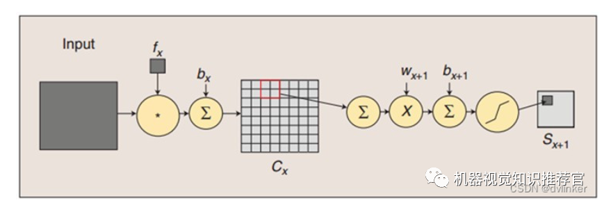
The convolution and subsampling processes are illustrated above. The convolution process involves using a trainable filter fx to convolve an input image (the first stage is the input image, and subsequent stages represent the convolved feature maps), then adding a bias bx to obtain the convolution layer Cx. The subsampling process includes summing the four pixels in each neighborhood to form one pixel, then weighting it with a scalar Wx+1 and adding bias bx+1, followed by a sigmoid activation function to produce a feature mapping that is roughly four times smaller.
Thus, the mapping from one plane to the next can be seen as performing convolution operations, while the S-layer can be viewed as a blurring filter, serving the purpose of secondary feature extraction. The spatial resolution decreases between hidden layers while the number of planes increases, allowing for the detection of more feature information.
The C3 layer is also a convolutional layer, which similarly convolves the S2 layer using a 5×5 convolution kernel, resulting in feature maps with only 10×10 neurons, but it has 16 different convolution kernels, hence 16 feature maps. It is important to note that each feature map in C3 is connected to all or several feature maps in S2, indicating that the feature maps in this layer are different combinations of the feature maps extracted in the previous layer.
As mentioned, each feature map in C3 is composed of combinations of all or several feature maps from S2. Why not connect each feature map in S2 to each feature map in C3? There are two reasons. First, the incomplete connection mechanism keeps the number of connections within a reasonable range. Second, and most importantly, it disrupts the symmetry of the network. Since different feature maps have different inputs, it forces them to extract different features.
For instance, one approach is that the first 6 feature maps in C3 take a subset of 3 adjacent feature maps from S2 as input. The next 6 feature maps take a subset of 4 adjacent feature maps from S2 as input. The following 3 take subsets of 4 non-adjacent feature maps. The last one takes all feature maps from S2 as input. Hence, the C3 layer has 1516 trainable parameters and 151600 connections.
The S4 layer is a subsampling layer, consisting of 16 feature maps of size 5*5. Each unit in the feature map is connected to the corresponding feature map’s 2*2 neighborhood in C3, similar to the connections between C1 and S2. The S4 layer has 32 trainable parameters (one factor and one bias for each feature map) and 2000 connections.
The C5 layer is a convolutional layer with 120 feature maps. Each unit is connected to the 5*5 neighborhood of all 16 units in the S4 layer. Since the size of the feature maps in S4 is also 5*5 (like the filter), the size of the C5 feature maps is 1*1, forming a fully connected layer between S4 and C5. The reason it is still labeled as a convolutional layer rather than a fully connected layer is that if the input to LeNet-5 increases in size while keeping everything else the same, the dimensions of the feature maps will exceed 1*1. The C5 layer has 48120 trainable connections.
The F6 layer has 84 units (the reason for choosing this number comes from the design of the output layer), and it is fully connected to the C5 layer. It has 10164 trainable parameters. Similar to classical neural networks, the F6 layer calculates the dot product between the input vector and the weight vector, adds a bias, and then passes it through the sigmoid function to produce the state of unit i.
Finally, the output layer consists of Euclidean Radial Basis Function (RBF) units, one for each class, each with 84 inputs. In other words, each RBF unit computes the Euclidean distance between the input vector and the parameter vector. The further the input is from the parameter vector, the larger the RBF output. An RBF output can be understood as a penalty term that measures the degree of match between the input pattern and the model associated with the RBF class. In probabilistic terms, the RBF output can be understood as the negative log-likelihood of the Gaussian distribution of the F6 layer’s configuration space. Given an input pattern, the loss function should ensure that the F6 configuration is close enough to the RBF parameter vector (i.e., the expected classification of the pattern). The parameters of these units are artificially selected and kept fixed (at least initially). The components of these parameter vectors are set to -1 or 1. Although these parameters can be randomly chosen with -1 and 1, or form an error correction code, they are designed to format an image of size 7*12 corresponding to a specific character class (i.e., 84). This representation is not very useful for recognizing individual digits but is useful for recognizing strings in the printable ASCII set.
Using this distributed coding rather than the more commonly used “1 of N” coding for generating output is another reason. When the number of categories is large, the performance of non-distributed coding is poor. The reason is that most of the time, the output of non-distributed coding must be 0. This makes it difficult to achieve with sigmoid units. Another reason is that the classifier is used not only for recognizing letters but also for rejecting non-letters. Using distributed coding RBF is more suited for this purpose because, unlike sigmoid, they excite well within the limiting regions of input space, while atypical patterns are more likely to fall outside.
The RBF parameter vector acts as the target vector for the F6 layer. It should be noted that the components of these vectors are +1 or -1, which is exactly within the range of the F6 sigmoid, thus preventing the saturation of the sigmoid function. In fact, +1 and -1 are the points of maximum curvature of the sigmoid function. This ensures that the F6 units operate within the maximum non-linear range. It is crucial to avoid the saturation of the sigmoid function, as this can lead to slow convergence of the loss function and pathological issues.
5.5. The Training Process
Neural networks for pattern recognition primarily use supervised learning networks, while unsupervised learning networks are more commonly used for clustering analysis. For supervised pattern recognition, since the category of each sample is known, the spatial distribution of samples is no longer divided according to their natural distribution tendencies but rather by finding an appropriate spatial partitioning method based on the distribution of similar samples in space and the degree of separation between different class samples, or finding a classification boundary that keeps different classes of samples in separate regions. This requires a long and complex learning process, continuously adjusting the position of the classification boundary used to partition the sample space, so as to minimize the number of samples classified into non-similar regions.
Convolutional networks are essentially a mapping from input to output, capable of learning a large number of mapping relationships between inputs and outputs without requiring any precise mathematical expression between inputs and outputs. As long as the convolutional network is trained with known patterns, it possesses the mapping capabilities between input-output pairs. The convolutional network undergoes supervised training, so its sample set consists of pairs of vectors in the form of (input vector, ideal output vector). All these vector pairs should originate from the actual “operational” results of the system that the network is about to simulate. They can be collected from the actual operating system. Before training begins, all weights should be initialized with different small random numbers. “Small random numbers” are used to ensure that the network does not enter a saturation state due to excessively large weights, which would lead to training failure; “different” ensures that the network can learn normally. In fact, if the same number is used to initialize the weight matrix, the network will have no learning capability.
The training algorithm is similar to the traditional BP algorithm. It mainly includes four steps, divided into two phases:
The first phase is the forward propagation phase:
a) Take a sample (X,Yp) from the sample set and input X into the network;
b) Calculate the corresponding actual output Op.
During this phase, information is transmitted from the input layer through successive transformations to the output layer. This process is also executed when the network runs normally after training. The network performs calculations (which essentially involve multiplying the input with the weight matrices of each layer to obtain the final output):
Op=Fn(…(F2(F1(XpW(1))W(2))…))W(n)
The second phase is the backward propagation phase:
a) Calculate the difference between the actual output Op and the corresponding ideal output Yp;
b) Adjust the weight matrix in reverse according to the method of minimizing error.
5.6. Advantages of Convolutional Neural Networks
Convolutional neural networks (CNNs) are primarily used to recognize two-dimensional graphics that exhibit invariance to translation, scaling, and other forms of distortion. Since the feature detection layers of CNNs learn from training data, explicit feature extraction is avoided, and learning occurs implicitly from the training data. Furthermore, since the weights of neurons on the same feature mapping plane are identical, the network can learn in parallel, which is a significant advantage of convolutional networks over networks where neurons are interconnected. With its unique structure of local weight sharing, convolutional neural networks have distinct advantages in speech recognition and image processing, as their layout is closer to actual biological neural networks. Weight sharing reduces the complexity of the network, particularly as multi-dimensional input vectors, such as images, can be directly input into the network, thereby avoiding the complexity of data reconstruction during feature extraction and classification.
Most classification methods are based on statistical features, which means that certain features must be extracted before differentiation. However, explicit feature extraction is not easy and is not always reliable in some application problems. Convolutional neural networks avoid explicit feature sampling and learn implicitly from training data. This makes convolutional neural networks significantly different from other neural network-based classifiers, integrating feature extraction capabilities into multilayer perceptrons through structural reorganization and weight reduction. They can directly handle grayscale images, making them suitable for image-based classification tasks.
Convolutional networks have the following advantages over traditional neural networks in image processing: a) The input image and the network topology can match well; b) Feature extraction and pattern classification occur simultaneously and are generated during training; c) Weight sharing can reduce the training parameters of the network, simplifying the neural network structure and enhancing adaptability.
6. Application Areas of Deep Learning
Deep learning is an important field of artificial intelligence with a wide range of applications, including but not limited to the following areas:
1) Image Recognition and Processing: Deep learning has many applications in image recognition, object detection, image segmentation, and facial recognition. Among them, deep learning models can learn from a large amount of data to recognize objects, scenes, faces, etc. in images, such as facial recognition technology, autonomous driving technology, and security monitoring.
2) Natural Language Processing: Deep learning has many applications in natural language processing, such as speech recognition, machine translation, text classification, sentiment analysis, etc. Through deep learning technologies, models can automatically understand the meaning and semantics of natural language based on the input natural language information, showing great application potential.
3) Human-Computer Interaction: Deep learning has many applications in human-computer interaction, such as intelligent customer service, intelligent question answering, and virtual characters. Through deep learning technologies, models can intelligently judge and respond based on user input, greatly helping people improve work and life efficiency.
4) Healthcare: Deep learning has many applications in healthcare, such as medical image analysis, disease diagnosis, and drug development. Through deep learning technologies, rapid disease diagnosis, assisting doctors in assessing conditions, and discovering new drugs can be accomplished.
5) Finance: Deep learning has many applications in finance, such as risk assessment, credit rating, and fraud detection. Through deep learning technologies, better recognition and analysis of changes and trends in financial markets can be achieved, enhancing financial risk control capabilities.
7. Achievements of Deep Learning Applications
Deep learning has been widely applied in fields such as search, data mining, computer vision, machine learning, machine translation, natural language processing, multimedia learning, speech, and personalized recommendations, achieving many application results.
7.1. In the Field of Computer Vision
Chinese University of Hong Kong’s Multimedia Laboratory is one of the earliest Chinese teams to apply deep learning in computer vision research. In the world-class AI competition LFW (Large-scale Face Recognition Competition), this laboratory outperformed Facebook to win the championship, marking the first time artificial intelligence surpassed human recognition capabilities in this field.
7.2. In the Field of Speech Recognition
Microsoft researchers first introduced RBM and DBN into the training of speech recognition acoustic models in collaboration with Hinton, achieving significant success in large vocabulary speech recognition systems, reducing the error rate of speech recognition by approximately 30%. However, DNN still lacks effective parallel fast algorithms, and many research institutions are using large-scale data corpora to improve the training efficiency of DNN acoustic models on GPU platforms.
Internationally, companies like IBM and Google have rapidly conducted DNN speech recognition research and are progressing swiftly.
Domestically, companies and research institutions such as Alibaba, iFlytek, Baidu, and the Chinese Academy of Sciences’ Automation Institute are also researching deep learning in speech recognition.
7.3. In Natural Language Processing and Other Fields
Many institutions are conducting research. In 2013, Tomas Mikolov, Kai Chen, Greg Corrado, and Jeffrey Dean published a paper titled Efficient Estimation of Word Representations in Vector Space, establishing the word2vector model, which can better express grammatical information compared to traditional bag-of-words models. Deep learning is primarily applied in natural language processing for machine translation and semantic mining.
In 2020, deep learning can accelerate innovation in semiconductor packaging and testing. In reducing repetitive manual tasks, improving yield, controlling precision and efficiency, and lowering inspection costs, AI deep learning-driven AOI has vast market potential, but mastering it is not simple.
On April 13, 2020, a study on medicine and artificial intelligence (AI) published in the journal Nature Machine Intelligence introduced an AI system that can scan cardiovascular blood flow in seconds. This deep learning model is expected to allow clinical physicians to observe blood flow changes in real-time while patients undergo MRI scans, thereby optimizing diagnosis workflows.
8. Summary of Deep Learning
Deep learning algorithms automatically extract the low-level or high-level features needed for classification. High-level features refer to features that can hierarchically depend on other features. For example, in machine vision, deep learning algorithms learn a low-level representation from the original image, such as edge detectors and wavelet filters, and then build expressions based on these low-level representations, such as linear or nonlinear combinations of these low-level representations, repeating this process to ultimately obtain a high-level representation.
Deep learning can obtain better representations of data features, and due to the model’s hierarchy and numerous parameters, it has sufficient capacity to represent large-scale data. Therefore, for problems where features are not obvious (requiring manual design and often lacking intuitive physical meaning), deep learning can achieve better results on large-scale training data. Additionally, from the perspective of feature recognition and classifiers, the deep learning framework integrates features and classifiers into one framework, learning features from data and reducing the massive workload of manually designing features (which is currently the most labor-intensive aspect for engineers in the industry). Therefore, not only can the results be better, but it is also much more convenient to use, making it a framework that deserves attention and that everyone in ML should understand.
Of course, deep learning itself is not perfect and is not a panacea for all ML problems; it should not be exaggerated to an all-powerful extent.
9. The Future of Deep Learning
Deep learning still has a lot of work to be researched. Current focuses are still borrowing methods from the field of machine learning that can be used in deep learning, especially in the area of dimensionality reduction. For example, one work involves sparse coding, using compressive sensing theory to reduce high-dimensional data, allowing a very small number of elements in a vector to accurately represent the original high-dimensional signal. Another example is semi-supervised learning, which projects the similarity of training samples into a low-dimensional space by measuring their similarity. Another promising direction is evolutionary programming approaches, which can perform conceptual adaptive learning and change core architectures by minimizing engineering energy.
Deep learning has achieved tremendous success in many fields, such as image recognition, natural language processing, and artificial intelligence. In the future, deep learning will continue to drive the development of artificial intelligence technology, bringing more convenience and innovation to humanity. Below are several trends for the future of deep learning:
1) Self-learning and self-optimization: As the complexity of deep learning models increases, how to enable models to learn and self-optimize better will become an important research area. Future deep learning models will be able to self-learn and adjust based on data, thereby improving accuracy and efficiency.
2) Integration of deep learning with sensor technology: With the development of the Internet of Things and sensor technology, deep learning will combine with sensor technology to achieve more intelligent applications. For example, deep learning can be used to solve issues such as traffic congestion, autonomous driving, and environmental monitoring.
3) Applications of deep learning in healthcare: Deep learning will become one of the important technologies in the healthcare field. Future deep learning models will be able to analyze and diagnose medical images, electronic medical records, and physiological data, helping doctors to diagnose and treat diseases faster.
4) Integration of deep learning with natural language processing: Deep learning will combine with natural language processing technology to achieve more efficient natural language processing and intelligent dialogue. Future deep learning models will be able to better understand language context and semantics, enabling more human-like interactions.
In summary, as deep learning technology continues to develop and advance, we can expect it to bring more innovation and change across various fields.
Copyright Statement: This article is an original piece by CSDN blogger “dvlinker” and follows the CC 4.0 BY-SA copyright agreement. Please include the original source link and this statement for any reprints.

END