Neural networks are an important machine learning technology. They form the basis of the currently hottest research direction—deep learning. Learning about neural networks not only allows you to master a powerful machine learning method but also helps you better understand deep learning technologies.
This article explains neural networks in a simple, step-by-step manner, suitable for those who have limited knowledge of neural networks. There are no specific prerequisites for reading this article, but having a basic understanding of machine learning will help in comprehending the content better.
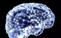
A neural network simulates the neural networks in the human brain to achieve artificial intelligence-like machine learning. The neural network in the human brain is a highly complex structure, with an estimated 100 billion neurons in an adult’s brain.
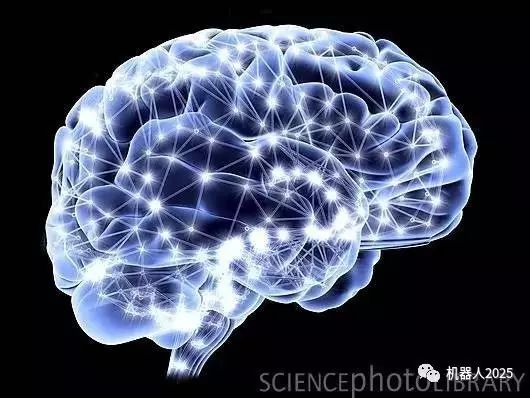 Figure 1: Neural Network of the Human Brain
So how do neural networks in machine learning achieve such impressive results? Through this article, you will find answers to these questions, as well as learn about the history of neural networks and how to study them effectively.
Due to the length of this article, here is a table of contents for the reader’s convenience:
1. Introduction
2. Neurons
3. Single-layer Neural Networks (Perceptron)
4. Two-layer Neural Networks (Multilayer Perceptron)
5. Multilayer Neural Networks (Deep Learning)
6. Review
7. Outlook
8. Conclusion
9. Afterword
10. Notes
1. Introduction
Let’s take a look at a classic neural network. This is a neural network consisting of three layers. The red layer is the input layer, the green layer is the output layer, and the purple layer is the hidden layer. The input layer has three input units, the hidden layer has four units, and the output layer has two units. In the following text, we will use this color scheme to represent the structure of the neural network.
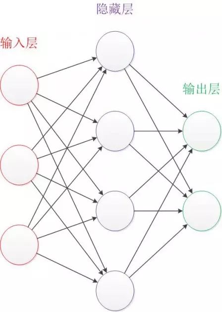
Figure 2: Structure of a Neural Network
Before we begin the introduction, there are some key points to keep in mind:
When designing a neural network, the number of nodes in the input and output layers is usually fixed, while the number of nodes in the hidden layer can be freely specified;
The topology and arrows in the neural network structure diagram represent the flow of data during the prediction process, which differs somewhat from the data flow during training;
The key in the structure diagram is not the circles (which represent “neurons”), but the connecting lines (which represent the connections between “neurons”). Each connecting line corresponds to a different weight (its value is called the weight), which needs to be learned during training.
In addition to the left-to-right representation, another common representation is bottom-to-top. In this case, the input layer is at the bottom of the diagram and the output layer is at the top, as shown in the following figure:
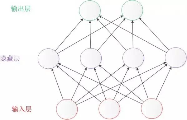
Figure 3: Bottom-to-top Structure of a Neural Network
The left-to-right representation is commonly used in the works of Andrew Ng and LeCun, while the bottom-to-top representation is used in Caffe. In this article, we will use the left-to-right representation as advocated by Andrew Ng.
Now, let’s start with the simple neuron and gradually introduce the complex structure of neural networks.
2. Neurons
1. Introduction
The study of neurons has a long history; as early as 1904, biologists understood the structural composition of neurons.
A neuron typically has multiple dendrites, primarily used to receive incoming information; while there is only one axon, which has many terminal branches that can transmit information to other neurons. The connection between the terminal branches and the dendrites of other neurons is called a synapse in biological terms.
The shape of neurons in the human brain can be simply illustrated in the following diagram:
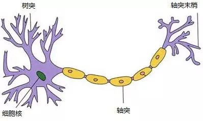
Figure 4: Neuron
In 1943, psychologist McCulloch and mathematician Pitts published an abstract model of a neuron called the MP model, referencing the structure of biological neurons. In the following text, we will introduce the neuron model in detail.
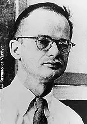
Figure 5: Warren McCulloch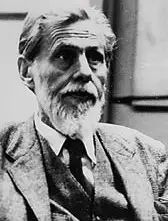 Walter Pitts
2. Structure
The neuron model is a model that includes input, output, and computational functions. The input can be likened to the dendrites of the neuron, while the output can be likened to the axon, and the computation can be likened to the cell nucleus.
The following diagram shows a typical neuron model: it contains three inputs, one output, and two computational functions.
Note the arrows in the middle. These lines are called “connections”. Each has a “weight” associated with it.
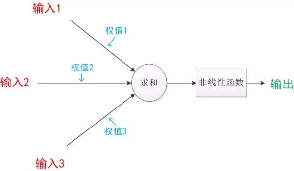
Figure 6: Neuron Model
Connections are the most important components of a neuron. Each connection has a weight.
The training algorithm of a neural network is to adjust the values of the weights to optimize the overall prediction performance of the network.
We denote the input as a and the weight as w. A directed arrow representing a connection can be understood as follows: at the starting point, the signal transmitted is still a, with a weighting parameter w in the middle, so the signal after weighting becomes a*w, thus at the end of the connection, the signal size becomes a*w.
In other drawing models, directed arrows may represent the unchanged transmission of values. However, in the neuron model, each directed arrow represents the weighted transmission of values.
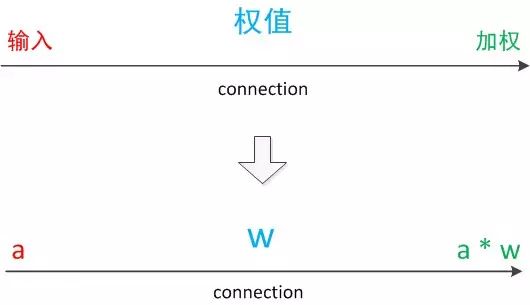
Figure 7: Connection
If we represent all the variables in the neuron diagram using symbols and write out the output calculation formula, it would look like the following:
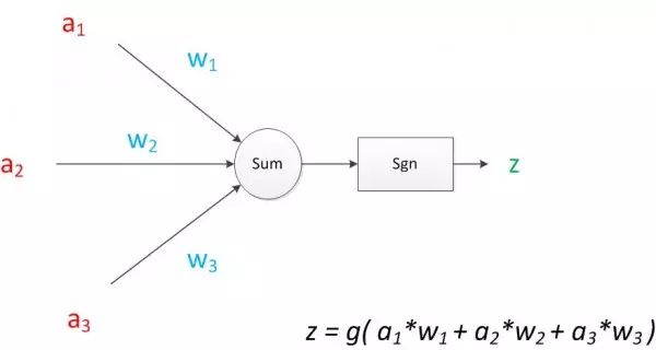
Figure 8: Neuron Calculation
It can be seen that z is the linear weighted sum of inputs and weights, plus a function g’s value. In the MP model, the function g is the sgn function, which is the sign function. This function outputs 1 when the input is greater than 0, otherwise, it outputs 0.
Next, we will expand the diagram of the neuron model. First, we will merge the sum function and the sgn function into a circle, representing the internal computation of the neuron. Second, we will write the inputs a and output z at the top left of the connection lines, making it easier to draw complex networks later. Finally, we note that a neuron can have multiple directed arrows representing outputs, but the values are the same.
A neuron can be seen as a computational and storage unit. The computation is the function that the neuron performs on its inputs. The storage is that the neuron temporarily stores the computed results and passes them to the next layer.
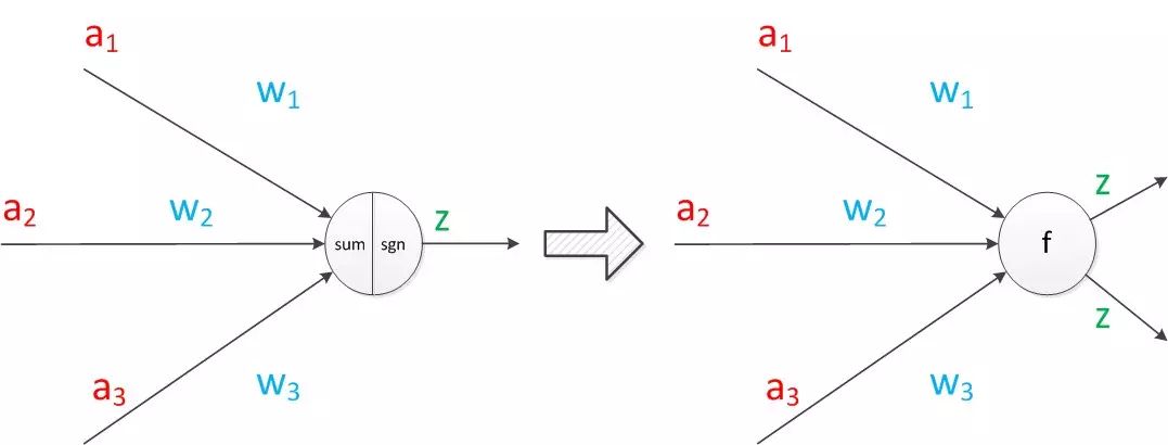
Figure 9: Expanded Neuron
When we construct a network of “neurons”, we often refer to a particular “neuron” in the network as a unit. Additionally, since the representation of neural networks is a directed graph, it is sometimes referred to as a node.
3. Effect
The use of the neuron model can be understood as follows:
We have a dataset, called a sample. The sample has four attributes, three of which are known, and one is unknown. What we need to do is predict the unknown attribute using the three known attributes.
The specific method is to use the neuron formula for computation. The known attribute values are a1, a2, a3, and the unknown attribute value is z. The value of z can be calculated using the formula.
Here, the known attributes are called features, and the unknown attribute is called the target. Assuming there is indeed a linear relationship between the features and the target, and we have obtained the weights w1, w2, w3 that represent this relationship, we can then predict the target of new samples using the neuron model.
4. Influence
The MP model published in 1943, though simple, laid the foundation for the neural network framework. However, in the MP model, the weights were all pre-set, so it could not learn.
In 1949, psychologist Hebb proposed the Hebb learning rate, suggesting that the strength of the synapses (i.e., connections) between neural cells in the brain can change. This led computational scientists to consider using weight adjustment methods for machine learning, laying the groundwork for subsequent learning algorithms.
Figure 10: Donald Olding Hebb
Although the neuron model and Hebb’s learning rule were born, due to the limitations of computer capabilities at that time, it was not until nearly a decade later that the first true neural network emerged.
3. Single-layer Neural Networks (Perceptron)
1. Introduction
In 1958, computational scientist Rosenblatt proposed a neural network composed of two layers of neurons, naming it the “Perceptron” (some literature translates it as “Perceptron”, but in this text, we will uniformly refer to it as “Perceptron”).
The Perceptron was the first artificial neural network that could learn. Rosenblatt demonstrated its learning process for recognizing simple images, which caused a sensation in society at that time.
People believed they had discovered the secrets of intelligence, and many scholars and research institutions invested in neural network research. The U.S. military heavily funded neural network research, considering it more important than the