

Author on Zhihu | Master Su
Link | https://zhuanlan.zhihu.com/p/139617364
This article introduces the visualization of the LSTM model structure.
Recently, I have been studying the application of LSTM in time series prediction, but I encountered a significant problem: after adding the time step to the traditional BP network, its structure becomes very difficult to understand, and the input-output data format is also hard to comprehend. There are many articles on LSTM structure online, but they are not intuitive and are very unfriendly to beginners. I also pondered for a long time, and only after looking at many materials and diagrams shared by netizens did I understand the intricacies. The content of this article is as follows:
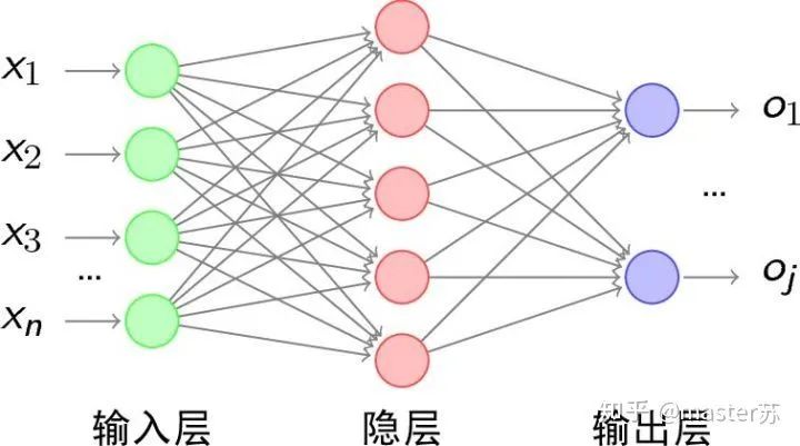
Traditional BP Networks and CNN Networks
BP networks and CNN networks do not have a time dimension, and they are similar to traditional machine learning algorithms. CNN can be understood as stacking multiple layers when processing the 3 channels of a color image. The three-dimensional matrix of the image can be understood as spatial slices, and when writing code, you can stack them layer by layer according to the diagram. The following figure shows a typical BP network and CNN network.
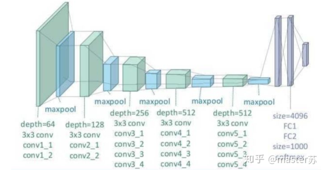
CNN Network
The hidden layers, convolutional layers, pooling layers, and fully connected layers in the figure all exist in reality, stacked layer by layer, which is easy to understand spatially. Therefore, when writing code, you basically look at the diagram to write the code. For example, using Keras:
# Sample code, no actual meaning
model = Sequential()
model.add(Conv2D(32, (3, 3), activation='relu'))  # Add convolutional layer
model.add(MaxPooling2D(pool_size=(2, 2)))         # Add pooling layer
model.add(Dropout(0.25))                          # Add dropout layer

model.add(Conv2D(32, (3, 3), activation='relu'))  # Add convolutional layer
model.add(MaxPooling2D(pool_size=(2, 2)))         # Add pooling layer
model.add(Dropout(0.25))                          # Add dropout layer
....   # Add other convolution operations
model.add(Flatten())                            # Flatten 3D array to 2D array
model.add(Dense(256, activation='relu'))        # Add a regular fully connected layer
model.add(Dropout(0.5))
model.add(Dense(10, activation='softmax'))
....  # Train the network
LSTM Networks
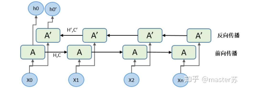
When we search for LSTM structures online, the most common image we see is the one below:
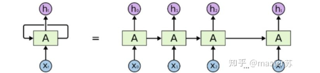
RNN Network
This is the classic structure diagram of the RNN recurrent neural network. LSTM is merely an improvement to the hidden layer node A, and the overall structure remains unchanged. Therefore, this article also discusses the visualization of this structure.
The A node in the hidden layer indicates that the left side represents an LSTM network with only one hidden layer. The so-called LSTM recurrent neural network utilizes cycles along the time axis, which is expanded into the right diagram when unfolded over the time axis.
Looking at the left diagram, many students believe that LSTM has a single input and single output, with only one hidden neuron in the network structure. However, looking at the right diagram, they think LSTM has multiple inputs and outputs, with multiple hidden neurons. The number of A represents the number of hidden layer nodes.
What the hell? It’s hard to switch thinking! This is the traditional network and spatial structure thinking.
In reality, in the right diagram, we see Xt representing the sequence, where the subscript t is the time axis. Therefore, the number of A indicates the length of the time axis, which is the state of the same neuron at different times (Ht), not the number of hidden layer neurons.
We know that the LSTM network uses the information from the previous moment, combined with the input information from the current moment, for joint training.
For example, on the first day, I got sick (initial state H0), then took medicine (using input information X1 to train the network), on the second day, I improved but was not completely well (H1), took medicine again (X2), and my condition improved (H2), and so forth until I recovered. Thus, the input Xt is taking medicine, the time axis T is the number of days taking medicine, and the hidden layer state is the condition. Therefore, I am still me, just in different states.
In fact, the LSTM network looks like this:
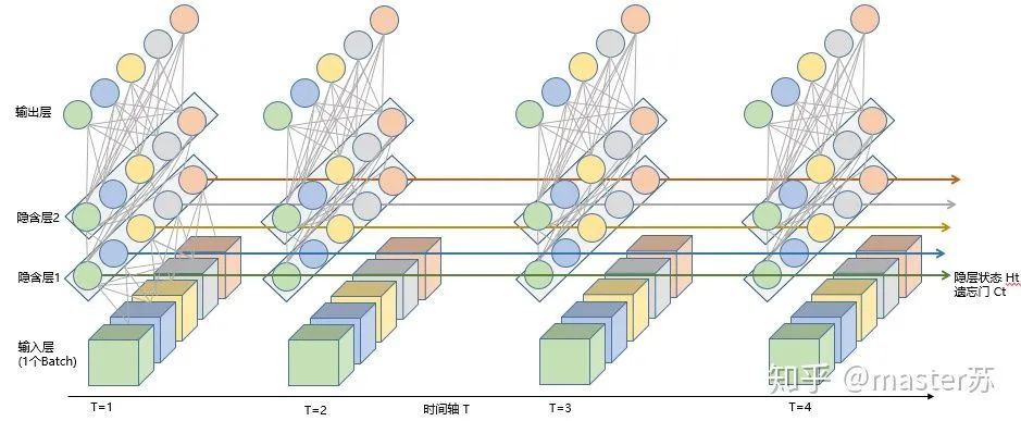
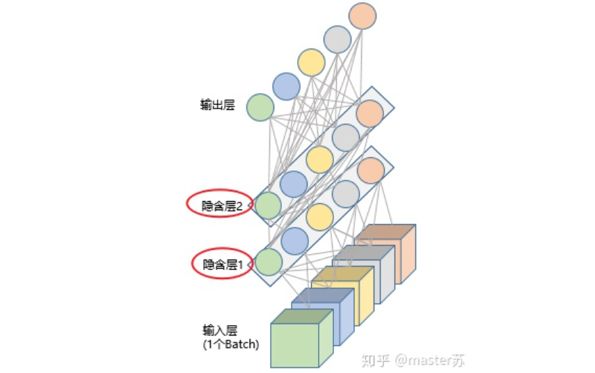
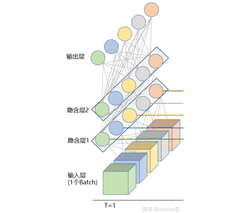
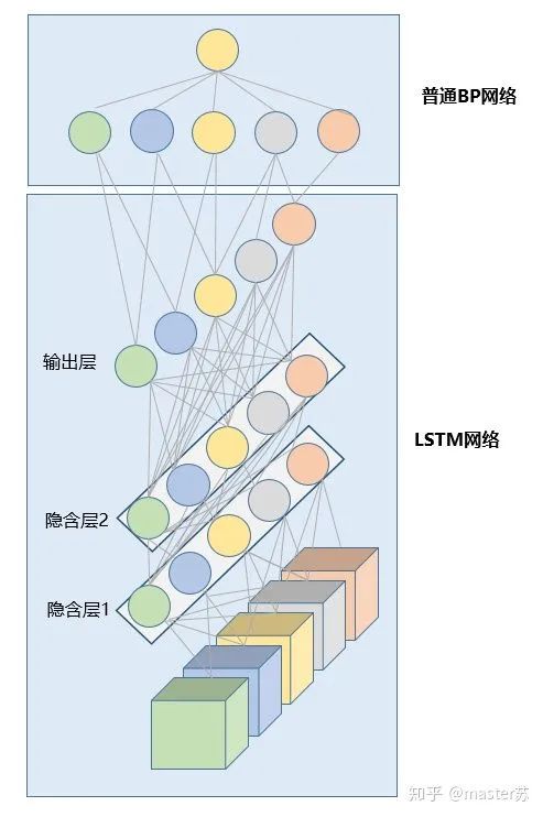
LSTM Network Structure
The above diagram represents an LSTM network with 2 hidden layers. At time T=1, it looks like a regular BP network, and at time T=2, it also appears as a regular BP network. However, the hidden layer information H and C trained at T=1 will be passed to the next moment T=2, as shown in the diagram below. The five arrows pointing to the right in the diagram also indicate the transmission of hidden layer states along the time axis.
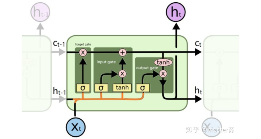
Note that in the diagram, H represents the hidden layer state, and C is the forget gate, which will be explained later in terms of their dimensions.
LSTM Input Structure
To better understand the LSTM structure, it is also necessary to understand the data input situation of LSTM. Following the example of a 3-channel image, the multi-sample, multi-feature data cube at different times with the time axis is shown in the diagram below:
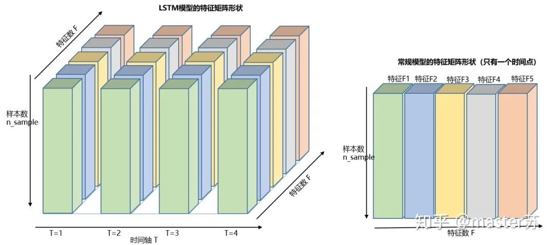
Three-Dimensional Data Cube
The diagram on the right shows the input format for commonly used models, such as XGBOOST, LightGBM, decision trees, etc., where the input data format is typically a (N*F) matrix. The left side, however, represents the data cube with the time axis added, which is a slice along the time axis, with dimensions (N*T*F). The first dimension is the number of samples, the second dimension is time, and the third dimension is the number of features, as shown in the diagram below:
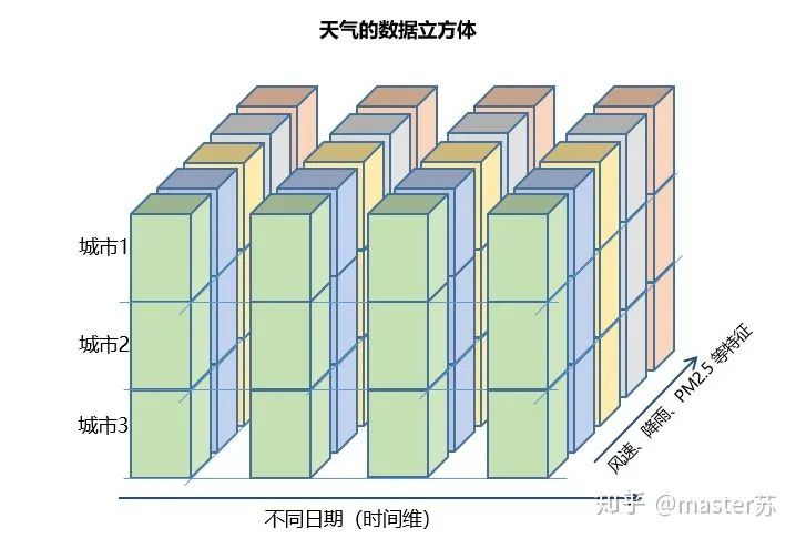
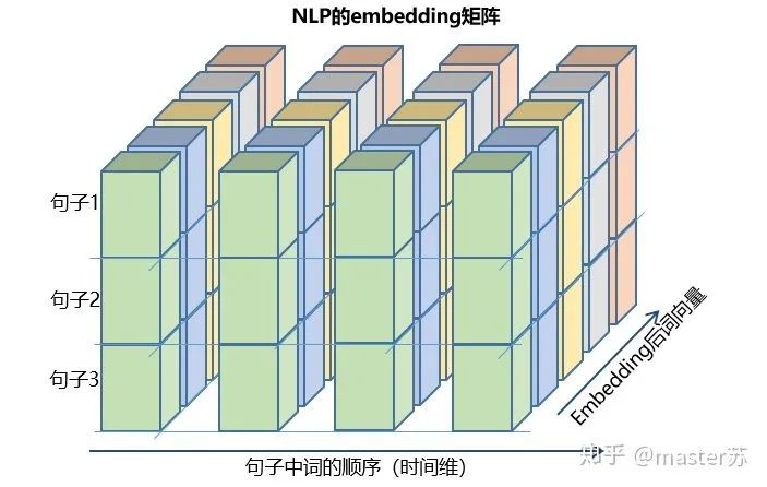
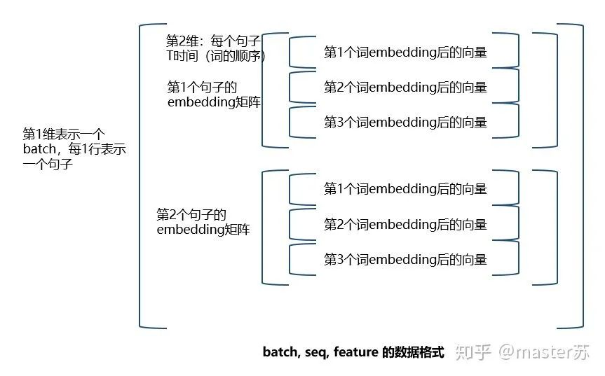
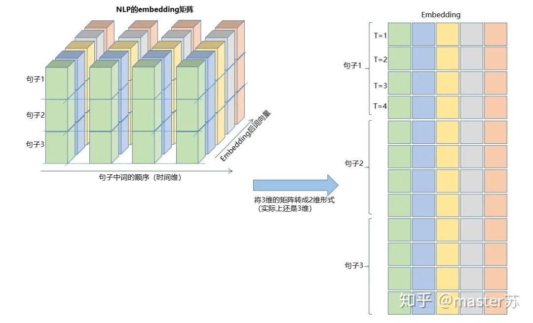
Such data cubes are abundant. For example, in weather forecasting data, samples can be understood as cities, the time axis is dates, and the features are weather-related factors such as rainfall, wind speed, PM2.5, etc. This data cube is easy to understand. In NLP, a sentence can be embedded into a matrix, where the order of words is the time axis T, and the embedding of multiple sentences can be represented as a three-dimensional matrix as shown below:
class torch.nn.LSTM(*args, **kwargs)
# Parameters:
# input_size: feature dimension of x
# hidden_size: feature dimension of the hidden layer
# num_layers: number of LSTM hidden layers, default is 1
# bias: If False, then bihbih=0 and bhhbhh=0. Default is True
# batch_first: If True, the input and output data format is (batch, seq, feature)
# dropout: Dropout is applied to the output of each layer except the last, default is 0
# bidirectional: If True, it is a bidirectional LSTM, default is False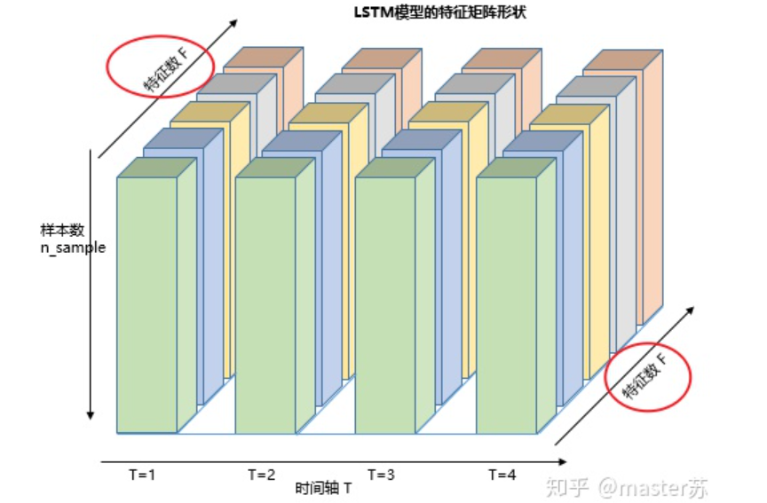
input(seq_len, batch, input_size)
# Parameters:
# seq_len: sequence length, in NLP it is the sentence length, usually padded with pad_sequence
# batch: the number of data entries fed to the network at once, in NLP it is how many sentences are fed to the network at once
# input_size: feature dimension, consistent with the input_size defined in the network structure.input(batch, seq_len, input_size)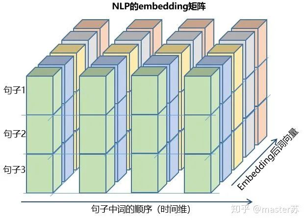
h0(num_layers * num_directions, batch, hidden_size)
c0(num_layers * num_directions, batch, hidden_size)
# Parameters:
# num_layers: number of hidden layers
# num_directions: if it is a unidirectional recurrent network, then num_directions=1, if bidirectional then num_directions=2
# batch: batch of input data
# hidden_size: number of hidden layer neuronsinput(batch, seq_len, input_size)h0(batch, num_layers * num_directions, hidden_size)
c0(batch, num_layers * num_directions, hidden_size)output, (ht, ct) = net(input)
# output: output of the hidden layer neurons at the last state
# ht: state value of the hidden layer at the last state
# ct: forget gate value of the hidden layer at the last stateoutput(seq_len, batch, hidden_size * num_directions)
ht(num_layers * num_directions, batch, hidden_size)
ct(num_layers * num_directions, batch, hidden_size)input(batch, seq_len, input_size)ht(batch, num_layers * num_directions, hidden_size)
ct(batch, num_layers * num_directions, hidden_size)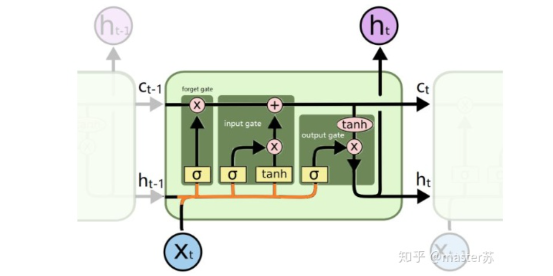
Implementing the above structure using PyTorch:
import torch
from torch import nn
class RegLSTM(nn.Module):
    def __init__(self):
        super(RegLSTM, self).__init__()
        # Define LSTM
        self.rnn = nn.LSTM(input_size, hidden_size, hidden_num_layers)
        # Define regression layer, input feature dimension equals LSTM output, output dimension is 1
        self.reg = nn.Sequential(
            nn.Linear(hidden_size, 1)
        )
    def forward(self, x):
        x, (ht, ct) = self.rnn(x)
        seq_len, batch_size, hidden_size = x.shape
        x = y.view(-1, hidden_size)
        x = self.reg(x)
        x = x.view(seq_len, batch_size, -1)
return xReference Links:
https://zhuanlan.zhihu.com/p/94757947
https://zhuanlan.zhihu.com/p/59862381
https://zhuanlan.zhihu.com/p/36455374
https://www.zhihu.com/question/41949741/answer/318771336
https://blog.csdn.net/android_ruben/article/details/80206792
Editor: Wang Jing
Proofread: Lin Yilin