Click the above“Beginner Learn Vision”, choose to addStar or “Top”

Important content delivered in real-time

The first convolutional neural network was proposed by Alexander Waibel in 1987, known as the Time Delay Neural Network (TDNN) [5]. TDNN is a convolutional neural network applied to speech recognition problems. It uses FFT to preprocess speech signals as input. Its hidden layers consist of two 1D convolution kernels to extract translational invariant features in the frequency domain [6]. Before the emergence of TDNN, there were breakthroughs in the research of backpropagation (BP) in the field of artificial intelligence [7], enabling TDNN to learn using the BP framework. In comparative experiments conducted by the original author, TDNN outperformed Hidden Markov Models (HMM), which were the mainstream algorithms for speech recognition in the 1980s [6].

In 1988, Zhang Wei proposed the first two-dimensional convolutional neural network, the Shift-Invariant Artificial Neural Network (SIANN), and applied it to medical image detection [1]. Yann LeCun also constructed a convolutional neural network for computer vision problems in 1989 [2], which is the original version of LeNet. LeNet consists of two convolutional layers and two fully connected layers, with a total of 60,000 learning parameters, far exceeding TDNN and SIANN, and its structure is very close to modern convolutional neural networks [4]. LeCun (1989) adopted [2] stochastic gradient descent (SGD) for weight learning after random initialization. This strategy has been retained in later deep learning institutions. Additionally, LeCun (1989) was the first to use the term convolution when discussing its network structure [2], naming it convolutional neural network.

For deep convolutional neural networks, after multiple convolutions and pooling, the final convolutional layer contains the richest spatial and semantic information. Each convolution unit in the convolutional neural network actually plays the role of an object detector, possessing the ability to locate objects, but the information contained is difficult for humans to understand and visualize.

In this article, we will review Class Activation Mapping (CAM), which draws on the ideas from the famous paper “Network In Network” by replacing the fully connected layer with Global Average Pooling (GAP).

The proposed CNN network has powerful image processing and classification capabilities, while also being able to locate key parts of the image.

Convolution Layers

Convolutional Neural Networks (CNN) mainly extract features continuously through a single filter, from local features to overall features, for image recognition and other functions.

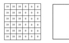
Assuming we need to process a single-channel grayscale image of size 6×6 pixels, we can convert it into a two-dimensional matrix as follows:

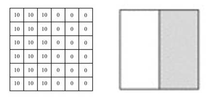
Source:https : //mc.ai/my-machine-learning-diary-day-68/

The numbers in the image represent the pixel values at that position; the larger the pixel value, the brighter the color. The boundary between the two colors in the middle of the image is the edge we want to detect.

We can design a filter (also known as a kernel) to detect this edge. Then, we will combine this filter with the input image to extract edge information, simplifying the convolution operation on the image into the following animation:

Source:https : //mc.ai/my-machine-learning-diary-day-68/

We cover the image with this filter, covering an area the same size as the filter, multiplying the corresponding elements, and then summing them up. After calculating one area, we move to another area and calculate until the entire original image is covered.

The output matrix is called a feature map, which is lighter in color in the middle and darker on the sides, reflecting the edges in the original image.

Source:https : //mc.ai/learning-to-perform-linear-filtering-using-natural-image-data/

The convolution layer mainly consists of two parts, a filter and a feature map. This is the first neural layer through which data flows in the CNN network. The more filters used in learning, the more features will be automatically adjusted in the CNN’s filter matrix.

Common hyperparameters to set include the number, size, and stride of filters.

Pooling

Pooling, also known as spatial pooling or subsampling, primarily functions to extract the main features of specific areas and reduce the number of parameters to prevent model overfitting.

No parameters need to be learned here. The hyperparameters to specify include the type of pooling, with common methods including Max pooling or Average pooling, window size, and stride. Typically, we use Max pooling more frequently, usually with a filter size of (2,2) and a stride of 2. After pooling, the input length and width will be reduced by half, and the channels will remain unchanged, as shown in the following diagram:

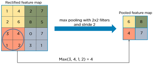
The maximum value is obtained within the pooling window and generates a new matrix after sequentially pooling on the feature map matrix. Similarly, we can also use averaging or summing methods, but typically, the results obtained using the maximum method are relatively better.

After several convolutions and pooling, we ultimately flatten the multidimensional data into a one-dimensional array and then connect them to the fully connected layer.

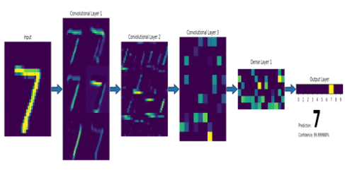
Source:https : //gfycat.com/fr/smoggylittleflickertailsquirrel-machine-learning-neural-networks-mnist

Its main function is to classify the processed images based on the feature set extracted through convolution and pooling layers.

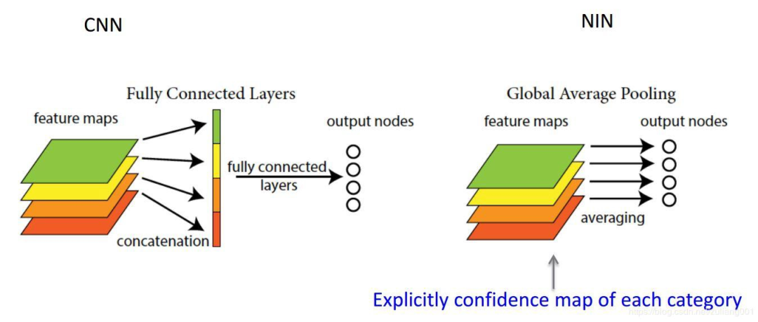
Fully convolutional networks like GoogleNet [10] avoid using fully connected layers and instead use Global Average Pooling (GAP). This not only reduces parameters to avoid overfitting but also creates feature maps associated with categories.

Global Average Pooling

For a long time, fully connected networks have been the standard structure for CNN classification networks. Typically, there will be an activation function for classification after fully connected layers. However, fully connected layers have a large number of parameters, which slows down training and makes it prone to overfitting.

The concept of Global Average Pooling was proposed in “Network In Network” [9] to replace fully connected layers.

Source:http : //www.programmersought.com/article/1768159517/

The difference between global average pooling and local average pooling is the pooling window. Local average pooling averages the values of subregions in the feature map, while in global average pooling, we average over the entire feature map.

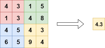
Source:https : //www.machinecurve.com/index.php/2020/01/30/what-are-max-pooling-average-pooling-global-max-pooling-and-global-average-pooling/

Using global average pooling instead of fully connected layers greatly reduces the number of parameters.

Class Activation Map

When using global average pooling, the final convolution layer is forced to generate as many feature maps as the number of categories we are targeting, which gives each feature map a very clear meaning, i.e., the class confidence map [11].

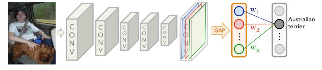
Source:https : //medium.com/@ahmdtaha/learning-deep-features-for-discriminative-localization-aa73e32e39b2

As seen in the image, after GAP, we obtain the average value of each feature map from the last convolution layer and derive the output through a weighted sum. For each category C, the average value of each feature map k has a corresponding weight w.

After training the CNN model, we can obtain a heat map to explain the classification result. For example, if we want to explain the classification result of class C, we take all the weights corresponding to class C and find their weighted sum corresponding to the feature maps. Since the size of this result is consistent with the feature maps, we need to upsample it and overlay it on the original image as shown below:

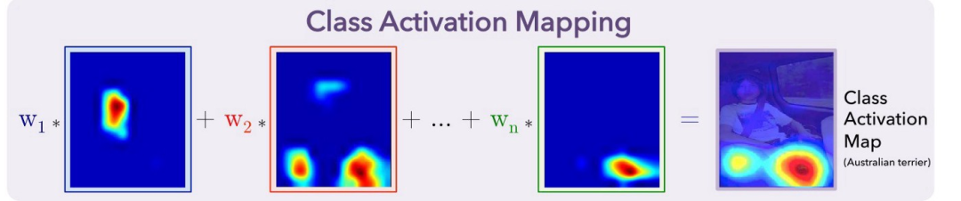
Source:https : //medium.com/@ahmdtaha/learning-deep-features-for-discriminative-localization-aa73e32e39b2

In this way, CAM tells us in the form of a heat map where the model focuses on the pixels used to determine the class C of the image.

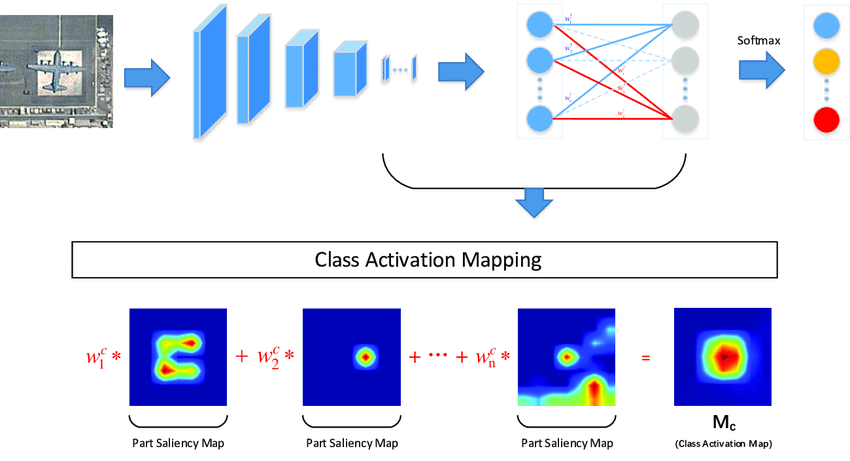
Source: MultiCAM: Multi-Class Activation Mapping for Aircraft Recognition in Remote Sensing Images

Conclusion

The explanation effect of CAM has always been good, but one drawback is that it requires modifying the structure of the original model, which leads to the need to retrain the model, greatly limiting its use cases. If the model is already online or the training cost is very high, it is almost impossible to retrain it.

Good news!<br/>Beginner Learn Vision Knowledge Circle<br/>Is now open to the public👇👇👇<br/><br/><br/>Download 1: OpenCV-Contrib Extension Module Chinese Version Tutorial<br/>Reply in the background of the "Beginner Learn Vision" public account: Extension Module Chinese Tutorial, you can download the first OpenCV extension module tutorial in the whole network, covering installation of extension modules, SFM algorithms, stereo vision, object tracking, biological vision, super-resolution processing, etc. over twenty chapters of content.<br/><br/>Download 2: Python Vision Practical Project 52 Lectures<br/>Reply in the background of the "Beginner Learn Vision" public account: Python Vision Practical Project, you can download 31 visual practical projects including image segmentation, mask detection, lane line detection, vehicle counting, eyeliner addition, license plate recognition, character recognition, emotion detection, text content extraction, facial recognition, etc., helping to quickly learn computer vision.<br/><br/>Download 3: OpenCV Practical Project 20 Lectures<br/>Reply in the background of the "Beginner Learn Vision" public account: OpenCV Practical Project 20 Lectures, you can download 20 practical projects based on OpenCV, achieving advanced learning of OpenCV.<br/><br/>Group Chat<br/><br/>Welcome to join the public account reader group to exchange with peers. Currently, there are WeChat groups for SLAM, 3D vision, sensors, autonomous driving, computational photography, detection, segmentation, recognition, medical imaging, GAN, algorithm competitions, etc. (will gradually subdivide in the future). Please scan the WeChat ID below to add to the group, and note: "Nickname + School/Company + Research Direction", for example: "Zhang San + Shanghai Jiao Tong University + Visual SLAM". Please follow the format for notes, otherwise you will not be approved. After successful addition, you will be invited to enter the relevant WeChat group based on your research direction. Please do not send advertisements in the group, otherwise you will be removed. Thank you for your understanding~