Click on the “MLNLP” above to select the “Star” public account
Heavyweight content delivered to you first
This article is the third in a series on decision trees, mainly introducing mainstream ensemble algorithms based on the Boosting framework, including XGBoost and LightGBM.
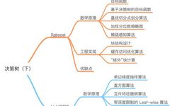
Here is the complete mind map:
XGBoost
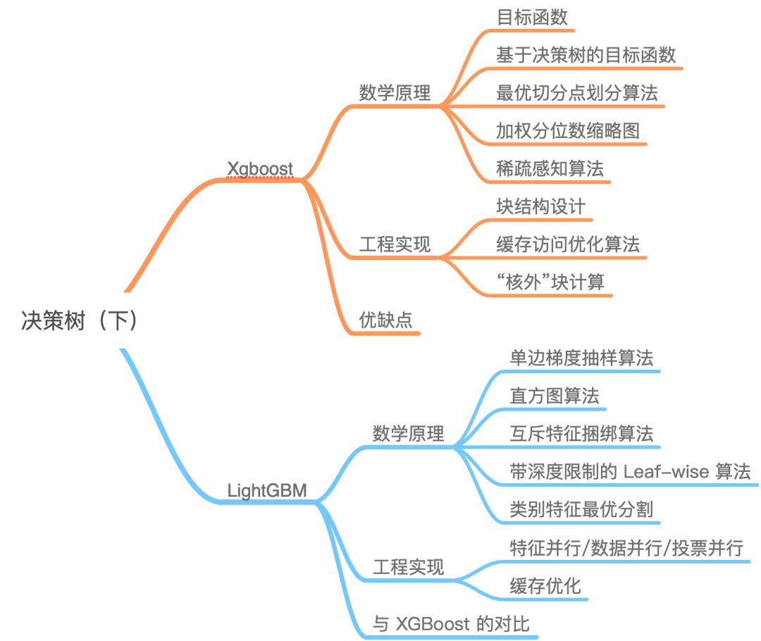
XGBoost is a tool for large-scale parallel boosting trees, currently the fastest and best open-source boosting tree toolkit, more than 10 times faster than common toolkits. Both XGBoost and GBDT are boosting methods, with the biggest difference being the definition of the objective function. Therefore, this article will introduce it from the mathematical principles and engineering implementations, and finally discuss the advantages of XGBoost.1.1 Mathematical Principles1.1.1 Objective FunctionWe know that XGBoost is an additive expression composed of k base models:where is the k-th base model, and is the predicted value of the i-th sample.The loss function can be represented by the predicted value and the true value :where n is the number of samples.We know that the predictive accuracy of the model is determined by both the bias and variance of the model, and the loss function represents the bias of the model. To have a low variance, a simpler model is needed, so the objective function is composed of the model’s loss function L and a regularization term that suppresses model complexity, so we have: is the regularization term of the model. Since XGBoost supports decision trees and linear models, it will not be described here.We know that the boosting model is forward additive. Taking the t-th step model as an example, the prediction of the i-th sample is:where is the predicted value given by the t-1 step model, which is a known constant, and is the predicted value of the new model we need to add this time. At this point, the objective function can be written as:Optimizing the objective function at this time is equivalent to solving .The Taylor formula is a method to approximate a function f(x) that has n derivatives at a point using an n-th polynomial about . If the function f(x) has n derivatives on a closed interval that contains , and has n+1 derivatives on an open interval (a,b), then for any point x on the closed interval , we have where the polynomial is called the Taylor expansion of the function at . The term is the remainder of the Taylor formula and is a high-order infinitesimal of .Based on the Taylor formula, we perform a second-order Taylor expansion of the function at point x, obtaining the following equality:We treat as and treat as , so we can write the objective function as:where is the first derivative of the loss function, and is the second derivative of the loss function. Note that the derivative here is taken with respect to .Taking the squared loss function as an example:we have:Since at step t, is actually a known value, so is a constant, and its optimization will not affect the function. Therefore, the objective function can be written as:Thus, we only need to find the first and second derivatives of the loss function at each step (since the previous step’s is known, these two values are constants), and then optimize the objective function to obtain the f(x) at each step. Finally, we can obtain an overall model based on the additive model.1.1.2 Objective Function Based on Decision TreesWe know that XGBoost’s base model supports not only decision trees but also linear models. Here we mainly introduce the objective function based on decision trees.We can define a decision tree as , where x is a certain sample. Here, q(x) represents which leaf node the sample is on, and w_q represents the value of the leaf node, so represents the value w for each sample (i.e., the predicted value).The complexity of the decision tree can be represented by the number of leaves T. The fewer the leaf nodes, the simpler the model. Additionally, the leaf nodes should not contain excessively high weights w (analogous to the weights of each variable in LR), so the regularization term of the objective function can be defined as:i.e., the complexity of the decision tree model is determined by the number of leaves of all generated decision trees and the L2 norm of the vector composed of the weights of all nodes.
This diagram illustrates how to solve the regularization term based on decision trees in XGBoost.We set as the sample set of the j-th leaf node, so our objective function can be written as:The second to third steps may not be very clear, so some explanation is provided here: the second step is to calculate the loss function for each sample after traversing all samples, but the samples will eventually fall into the leaf nodes, so we can also traverse the leaf nodes and obtain the sample set on the leaf nodes, and then calculate the loss function.That is, the sample set we had before is now rewritten as the set of leaf nodes. Since a leaf node can contain multiple samples, there are and terms, where is the value of the j-th leaf node.To simplify the expression, we define , so the objective function becomes:Here we must note that and are the results obtained from the previous t-1 steps, their values are known and can be treated as constants, only the leaf node of the last tree is uncertain. Then, taking the first derivative of the objective function with respect to and setting it to 0, we can obtain the weight corresponding to the leaf node j:Thus, the objective function can be simplified as:
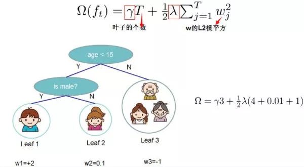
The above figure provides an example of calculating the objective function, requiring the first and second derivatives and for each node and sample, and then summing and for each node containing samples to finally traverse the nodes of the decision tree to obtain the objective function.1.1.3 Optimal Split Point Division AlgorithmA very critical issue in the growth of decision trees is how to find the optimal split point of the leaf nodes. XGBoost supports two methods for splitting nodes—greedy algorithm and approximate algorithm.1) Greedy Algorithm
Starting with a tree of depth 0, enumerate all available features for each leaf node;
For each feature, sort the training samples belonging to that node in ascending order based on the feature value, and determine the best split point for that feature through linear scanning, recording the split gain for that feature;
Select the feature with the highest gain as the splitting feature, use the best split point of that feature as the split position, split the node into two new leaf nodes, and associate the corresponding sample set with each new node;
Return to step 1, recursively execute until a specific condition is met;
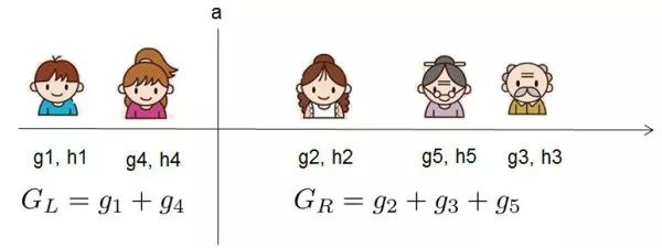
So how do we calculate the split gain for each feature?Suppose we complete the feature split at a certain node, then the objective function before splitting can be written as:The objective function after splitting is:Then the gain from the split for the objective function is:Note that the gain of the feature can also serve as an important basis for feature importance output.For each split, we need to enumerate all possible splitting schemes for the features. How can we efficiently enumerate all splits?I assume we want to enumerate all conditions such as x < a. For a specific split point a, we need to calculate the sum of gradients on the left and right of a.
We can see that for all split points a, we only need to perform a left-to-right scan to enumerate all the gradient sums and . Then we can use the above formula to calculate the score for each split scheme.2) Approximate AlgorithmThe greedy algorithm can obtain the optimal solution, but when the data volume is too large, it cannot be loaded into memory for computation. The approximate algorithm mainly provides an approximate optimal solution for this shortcoming of the greedy algorithm.For each feature, only considering quantiles can reduce computational complexity.This algorithm first proposes candidate split points based on the quantiles of the feature distribution, then maps continuous features into buckets defined by these candidate points, and finally aggregates statistical information to find the best split point for all intervals.When proposing candidate split points, there are two strategies:
Global:Candidate split points are proposed before learning each tree, and this split is adopted every time a split is made;
Local:Candidate split points are proposed again before each split;
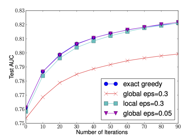
Intuitively, the Local strategy requires more computational steps, while the Global strategy requires more candidate points since nodes are not divided.The following figure shows the AUC transformation curves for different splitting strategies, where the horizontal axis is the number of iterations and the vertical axis is the AUC for the test set. eps is the accuracy of the approximate algorithm, and its reciprocal is the number of buckets.
We can see that the Global strategy can achieve similar accuracy to the Local strategy when the number of candidate points is large (eps small) and the Local strategy when the number of candidate points is small (eps large).Additionally, we also find that when eps is reasonably set, the quantile strategy can achieve the same accuracy as the greedy algorithm.
The first for loop:Find the candidate set of cutting points for feature k based on the quantiles of that feature distribution.XGBoost supports both Global and Local strategies.
The second for loop:For the candidate set of each feature, map the samples into buckets defined by the candidate points corresponding to that feature, that is , and for each bucket, count G and H values, and finally find the best split point based on these statistics.
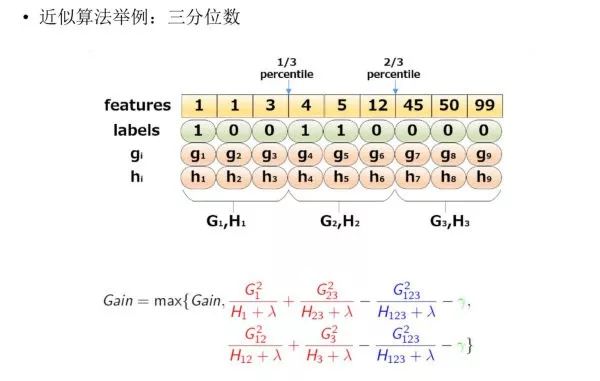
The following figure provides a specific example of the approximate algorithm, taking the quartiles as an example:
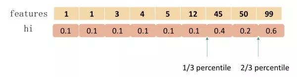
Based on the sample features, sorting, and then dividing based on quantiles, counting the G and H values within the three buckets, and finally solving for the gain of the node division.1.1.4 Weighted Quantile SketchIn fact, XGBoost does not simply perform quantiles based on the number of samples but uses the second derivative value as the weight of the samples for splitting, as follows:
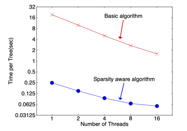
Then the question arises:Why use for sample weighting?We know that the model’s objective function is:With slight rearrangement, we can see that has the effect of weighting the loss.Where and C are both constants.We can see that h_i is the weight of the samples in the squared loss function.For datasets where sample weights are the same, there is already a solution for finding candidate quantile points (the GK algorithm), but how do we find candidate quantile points when sample weights are different?(The author provides a Weighted Quantile Sketch algorithm, which will not be introduced here.)1.1.5 Sparse-Aware AlgorithmIn the first article on decision trees, we introduced the splitting strategy of the CART tree when dealing with missing data, and XGBoost also provides its solution.XGBoost only considers non-missing values during the traversal of data for constructing tree nodes, and adds a default direction for each node. When the corresponding feature value of a sample is missing, it can be classified into the default direction, and the optimal default direction can be learned from the data.As for how to learn the branches of the default values, it is actually very simple. Enumerate the gains when the feature is missing for left and right branches, and choose the one with the highest gain as the optimal default direction.During the tree-building process, it is necessary to enumerate samples with missing features. At first glance, this algorithm seems to double the computational load, but in fact, this algorithm only considers traversing samples with non-missing features during the tree-building process, and samples with missing feature values do not need to be traversed; they can be directly assigned to the left and right nodes. Therefore, the number of samples that need to be traversed by the algorithm is reduced. The following figure shows that the sparse-aware algorithm is more than 50 times faster than the basic algorithm.
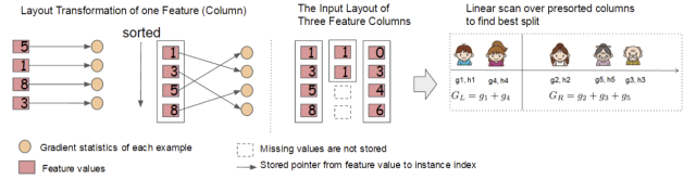
1.2 Engineering Implementation1.2.1 Block Structure DesignWe know that the most time-consuming step in learning decision trees is sorting the feature values each time to find the best split point.XGBoost sorts the data based on features before training and saves it to a block structure, using a sparse matrix storage format (Compressed Sparse Columns Format, CSC) in each block structure. The training process will repeatedly use the block structure, which can greatly reduce the computational load.
Each block structure contains one or more already sorted features;
Missing feature values will not be sorted;
Each feature will store an index pointing to the sample gradient statistics, facilitating the calculation of first and second derivative values;
This block structure allows the features to be independent of each other, facilitating parallel computation by the computer. When splitting nodes, the feature with the highest gain needs to be selected for splitting, and at this point, the gain calculations for each feature can be performed simultaneously. This is also the reason why XGBoost can achieve distributed or multithreaded computation.1.2.2 Cache Access Optimization AlgorithmThe design of the block structure can reduce the computational load during node splitting, but the design of accessing sample gradient statistics through index can lead to non-continuous memory space for access operations, which can result in low cache hit rates and thus affect the efficiency of the algorithm.To solve the problem of low cache hit rates, XGBoost proposes a cache access optimization algorithm: Allocate a continuous cache area for each thread, storing the required gradient information in the buffer, thus achieving the conversion from non-continuous space to continuous space, improving algorithm efficiency.Additionally, appropriately adjusting block sizes can also help optimize the cache.1.2.3 “Out-of-Core” Block ComputationWhen the data volume is too large to load all the data into memory, it can only temporarily store data that cannot be loaded into memory on the hard disk, and load it for computation when needed. This operation inevitably involves resource waste and performance bottlenecks due to the speed differences between memory and hard disk.To address this issue, XGBoost dedicates a thread specifically for reading data from the hard disk to achieve simultaneous data processing and data reading.Furthermore, XGBoost has also used two methods to reduce the overhead of hard disk read and write:
Block compression:Compress blocks by columns and decompress them during reading;
Block splitting:Store each block on different disks, increasing throughput by reading from multiple disks.
1.3 Advantages and Disadvantages1.3.1 Advantages
Higher accuracy:GBDT only uses the first-order Taylor expansion, while XGBoost performs a second-order Taylor expansion on the loss function.XGBoost introduces the second derivative to increase accuracy and also to allow for custom loss functions. The second-order Taylor expansion can approximate a large number of loss functions;
Greater flexibility:GBDT uses CART as the base classifier, while XGBoost supports not only CART but also linear classifiers (using linear classifiers with XGBoost is equivalent to logistic regression with L1 and L2 regularization terms for classification problems or linear regression for regression problems).Additionally, the XGBoost tool supports custom loss functions, as long as the function supports first and second derivatives;
Regularization:XGBoost adds regularization terms to the objective function to control model complexity.The regularization term includes the number of leaf nodes in the trees and the L2 norm of the weights of the leaf nodes.The regularization term reduces the variance of the model, making the learned model simpler and helping to prevent overfitting;
Shrinkage:Equivalent to learning rate.After each iteration, XGBoost multiplies the weights of the leaf nodes by this coefficient, mainly to weaken the influence of each tree, allowing for greater learning space for subsequent trees;
Column sampling:XGBoost adopts the approach of random forests, supporting column sampling, which can reduce overfitting and computational costs;
Handling missing values:The sparse-aware algorithm used by XGBoost greatly speeds up the node splitting process;
Although pre-sorting and approximate algorithms can reduce the computational load of finding the best split points, the dataset still needs to be traversed during node splitting;
The space complexity of the pre-sorting process is too high, requiring not only storage for feature values but also for the indices of the gradient statistics corresponding to the features, effectively consuming double the memory.
LightGBM
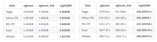
LightGBM, proposed by Microsoft, is mainly used to solve the problems encountered by GDBT in massive data, so that it can be better and faster used in industrial practice.From the name LightGBM, we can see that it is a lightweight (Light) gradient boosting machine (GBM), which has faster training speed and lower memory usage compared to XGBoost.The following figure shows the comparison of memory and training time between XGBoost, XGBoost_hist (XGBoost using gradient histogram), and LightGBM under different datasets:
So how does LightGBM achieve faster training speed and lower memory usage?We have just analyzed the disadvantages of XGBoost; to address these issues, LightGBM proposes the following solutions:
Gradient-based One-Side Sampling algorithm;
Histogram algorithm;
Exclusive Feature Bundling algorithm;
Leaf-wise vertical growth algorithm based on maximum depth;
Optimal splitting for categorical features;
Feature parallelism and data parallelism;
Cache optimization.
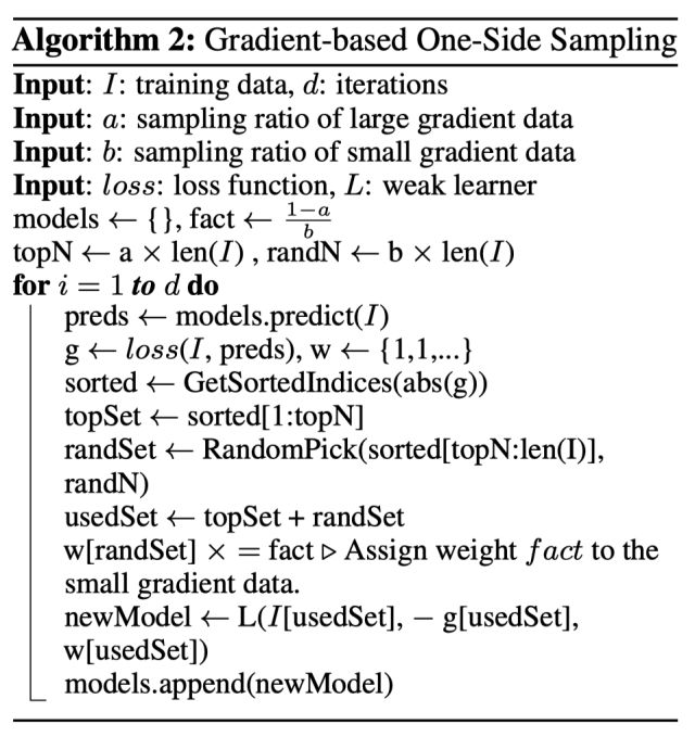
This section will continue to introduce LightGBM from both mathematical principles and engineering implementations.2.1 Mathematical Principles2.1.1 Gradient-based One-Side Sampling AlgorithmThe gradient size of the GBDT algorithm can reflect the weight of the samples. A smaller gradient indicates better model fitting. The Gradient-based One-Side Sampling (GOSS) algorithm utilizes this information to sample the samples, reducing a large number of samples with small gradients, focusing only on samples with high gradients in subsequent calculations, greatly reducing computational load.The GOSS algorithm retains samples with large gradients and randomly samples those with small gradients. To avoid changing the data distribution, a constant is introduced for balancing when calculating gains for samples with small gradients.The specific algorithm is as follows:
We can see that GOSS first sorts samples based on the absolute value of gradients (without saving the sorted results) and then takes the top a% of samples with large gradients and b% of the remaining samples. When calculating gains, the weights of the samples with small gradients are amplified by multiplying by rac{1-a}{b}.On one hand, the algorithm focuses more on underfitted samples, and on the other hand, it prevents sampling from having too much impact on the original data distribution by multiplying weights.2.1.2 Histogram Algorithm
Histogram Algorithm
The basic idea of the histogram algorithm is to discretize continuous features into k discrete features while constructing a histogram with a width of k to gather statistical information (containing k bins).Using the histogram algorithm, we do not need to traverse the data; we only need to traverse the k bins to find the best split point.We know that discretizing features has many advantages, such as easier storage, faster computation, stronger robustness, and more stable models.For the histogram algorithm, the most direct benefits include the following two (taking k=256 as an example):
Lower memory usage:XGBoost needs to store feature values with 32-bit floating-point numbers and store indices with 32-bit integers, while LightGBM only needs 8 bits to store histograms, effectively reducing the usage to 1/8;
Lower computational cost:When calculating feature split gains, XGBoost needs to traverse the data once to find the best split point, while LightGBM only needs to traverse k times, directly reducing the time complexity from O(#data * #feature) to O(k * #feature), where we know #data >> k.
Although discretizing features may not find the exact split points, it may have some impact on model accuracy, but the coarser splits also serve as a form of regularization, reducing the model’s variance to some extent.
Histogram Acceleration
When constructing the histogram of leaf nodes, we can also build it by subtracting the histograms of parent nodes and adjacent leaf nodes, thereby reducing computational load by half.In practice, we can first compute the histograms of smaller leaf nodes and then use the histogram difference to obtain the histograms of larger leaf nodes.
Sparse Feature Optimization
XGBoost only considers non-zero values during pre-sorting for acceleration, while LightGBM adopts a similar strategy: Only use non-zero features to construct histograms.2.1.3 Exclusive Feature Bundling AlgorithmHigh-dimensional features are often sparse, and features may be mutually exclusive (e.g., two features cannot take non-zero values simultaneously). If two features are not completely exclusive (e.g., only a part of the time do they not take non-zero values), we can use mutual exclusivity to represent the degree of exclusiveness.The Exclusive Feature Bundling (EFB) algorithm states that if some features are fused together, the number of features can be reduced.In addressing this idea, we encounter two questions:
Which features can be bundled together?
After feature bundling, how to determine the feature values?
For the first question:The EFB algorithm constructs a weighted undirected graph based on the relationships between features and converts it to a graph coloring algorithm.We know that graph coloring is an NP-Hard problem, so a greedy algorithm is used to obtain an approximate solution, with the following steps:
Construct a weighted undirected graph, where vertices are features, and edges represent the degree of mutual exclusivity between two features;
Sort the nodes in descending order based on their degree; the higher the degree, the greater the conflict with other features;
Traverse each feature, assigning it to an existing feature bundle or creating a new feature bundle to minimize overall conflict.
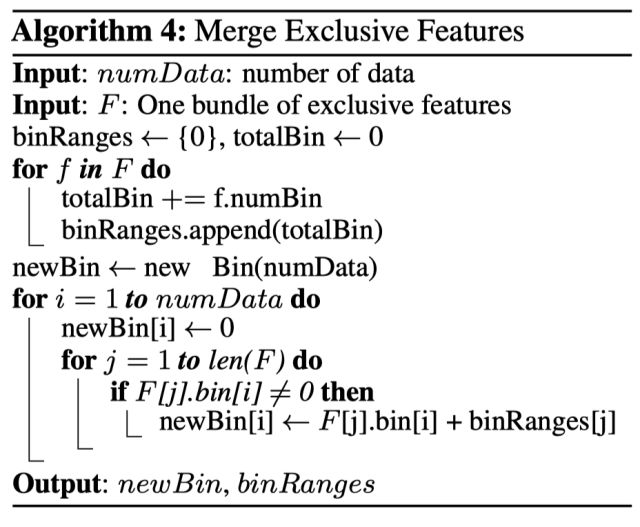
The algorithm allows for pairs of features that are not completely exclusive to increase the number of feature bundles by setting a maximum mutual exclusivity rate to balance the algorithm’s accuracy and efficiency. The pseudocode for the EFB algorithm is as follows:
We see that the time complexity is O(#feature^2). In cases where the number of features is not high, this can be managed, but if the feature dimension reaches millions, the computational load will be significant. To improve efficiency, we propose a faster solution: Change the strategy of sorting based on node degree in the EFB algorithm to sorting based on the number of non-zero values since the more non-zero values, the higher the probability of mutual exclusivity.For the second question:The paper presents a feature merging algorithm, which is key to ensuring that original features can be separated from merged features.Assuming there are two feature values in a Bundle, A takes values [0, 10] and B takes values [0, 20], to ensure the exclusivity of features A and B, we can add an offset to feature B to convert it to [10, 30]. The merged feature would then take values [0, 30], thus achieving feature merging.The specific algorithm is as follows:
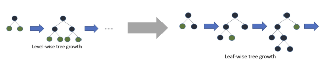
2.1.4 Leaf-wise Algorithm with Depth LimitationIn the process of building trees, there are two strategies:
Level-wise:Growth based on levels until stopping conditions are met;
Leaf-wise:Split the leaf node with the highest gain each time until stopping conditions are met.
XGBoost adopts a Level-wise growth strategy, facilitating parallel computation of each layer’s splitting nodes, improving training speed, but it also increases unnecessary splits due to low node gains, reducing computational efficiency.LightGBM adopts a Leaf-wise growth strategy to reduce computational load, combined with maximum depth limitations to prevent overfitting. However, since it always computes the node with the highest gain, it cannot split in parallel.
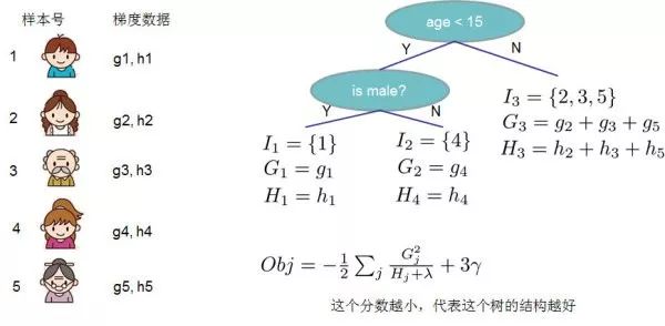
2.1.5 Optimal Splitting for Categorical FeaturesMost machine learning algorithms do not directly support categorical features and generally encode categorical features before inputting them into the model.The common method for handling categorical features is one-hot encoding, but we know that one-hot encoding is not recommended for decision trees:
It can lead to sample splitting imbalance, resulting in very small split gains.For example, nationality splits can create features like whether it is China, whether it is the USA, etc., where only a small number of samples are 1 and a large number of samples are 0.This kind of split gain is very small:The smaller split sample set occupies too small a proportion of the total sample.No matter how large the gain is, after multiplying by that proportion, it can almost be ignored;The larger split sample set is almost the original sample set, with nearly zero gain;
Affecting decision tree learning:Decision trees rely on statistical information of data, and one-hot encoding scatters data into small spaces.In these scattered small spaces, the statistical information is inaccurate, leading to poorer learning outcomes.The essence is that the expressiveness of features after one-hot encoding is poor; the predictive capability of features is artificially split into multiple parts, each competing for optimal split points fails, resulting in the importance of that feature being lower than its actual value.
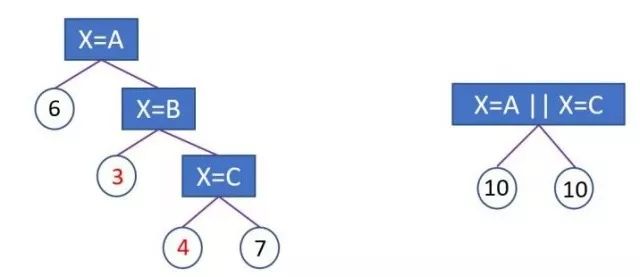
LightGBM natively supports categorical features, adopting a many-vs-many splitting method to achieve optimal splitting for categorical features.Assuming a certain dimension feature has k categories, there are 2^{(k-1)} – 1 possibilities, with a time complexity of O(2^k). LightGBM implements a time complexity of O(klog_2k) based on Fisher’s paper “On Grouping For Maximum Homogeneity”.
The left image shows splitting based on one-hot encoding, while the right image shows LightGBM splitting based on many-vs-many. Under a given depth, the latter can learn a better model.The basic idea is that each time a grouping is performed, the categorical features are classified based on the training objective, sorting the histogram based on their cumulative values rac{ ext{sum gradient}}{ ext{sum hessian}}, and then finding the best split on the sorted histogram.Additionally, LightGBM also adds regularization constraints to prevent overfitting.
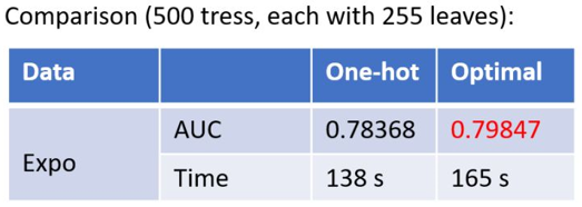
We can see that this method of handling categorical features increased the AUC by 1.5 points, with only a 20% increase in time.2.2 Engineering Implementation2.2.1 Feature ParallelismThe traditional feature parallel algorithm involves vertically partitioning data, then using different machines to find optimal splitting points for different features, integrating the best splitting points based on communication, and then informing other machines of the splitting results.The traditional feature parallel method has a significant drawback:It requires informing each machine of the final splitting results, increasing additional complexity (because the data is vertically partitioned, each machine has different data, the splitting results need to be communicated).LightGBM does not perform vertical data partitioning; each machine has the complete training set. After obtaining the best splitting scheme, the splitting can be executed locally, reducing unnecessary communication.2.2.2 Data ParallelismThe traditional data parallel strategy mainly involves horizontally partitioning data, then locally constructing histograms and integrating them into a global histogram, finally finding the optimal splitting point in the global histogram.This data partitioning has a significant drawback:Excessive communication overhead.If using point-to-point communication, the communication overhead for one machine is approximately O(#machine * #feature *#bin);If using integrated communication, the communication overhead is O(2 * #feature *#bin);LightGBM adopts a distributed reduction (Reduce scatter) approach to distribute the task of histogram integration across different machines, thereby reducing communication costs and further lowering communication between different machines through histogram differences.2.2.3 Voting ParallelismFor cases where the data volume is particularly large and features are numerous, voting parallelism can be adopted.Voting parallelism mainly optimizes the bottleneck of communication costs during data parallelism by only merging histograms of a subset of features to reduce communication volume.The general steps are two:
Locally identify the Top K features and use voting to select features that are likely to be optimal splitting points;
During merging, only merge the features selected by each machine.
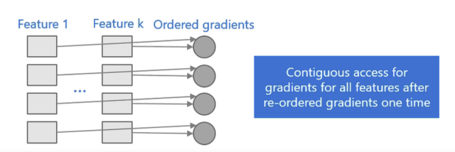
2.2.4 Cache OptimizationAs mentioned earlier, XGBoost’s pre-sorted features provide indices for the sample gradient statistics, which can lead to non-continuous access results. XGBoost proposes a cache access optimization algorithm for improvement.In contrast, the histogram algorithm used by LightGBM is inherently cache-friendly:
First, all features use the same method to obtain gradients (unlike different features obtaining gradients through different indices), allowing for sorted gradients and achieving continuous access, greatly improving cache hits;
Secondly, since there is no need to store indices of features to samples, storage consumption is reduced, and there are no Cache Miss issues.
2.3 Comparison with XGBoostThis section mainly summarizes the advantages of LightGBM compared to XGBoost, introducing them from the perspectives of memory and speed.2.3.1 Smaller Memory
XGBoost requires recording feature values and their corresponding sample statistics indices after pre-sorting, while LightGBM uses the histogram algorithm to convert feature values into bin values, and does not need to record indices of features to samples, reducing space complexity from O(2*#data) to O(#bin), significantly decreasing memory consumption;
LightGBM adopts the histogram algorithm to convert storage of feature values into storage of bin values, reducing memory consumption;
LightGBM reduces the number of features during training through the exclusive feature bundling algorithm, decreasing memory consumption.
2.3.2 Faster Speed
LightGBM uses the histogram algorithm to convert sample traversal into histogram traversal, significantly reducing time complexity;
LightGBM filters out samples with small gradients during training using the one-sided gradient algorithm, reducing a large amount of computation;
LightGBM adopts a leaf-wise growth strategy to build trees, reducing many unnecessary computations;
LightGBM accelerates computation through optimized feature parallelism and data parallelism methods, and can also use voting parallelism when the data volume is very large;
LightGBM also optimizes cache, increasing the hit rate of Cache hits.
References
XGBoost: A Scalable Tree Boosting System
Chen Tianqi’s paper presentation PPT
What are the differences between GBDT and XGBOOST in machine learning algorithms? – wepon’s answer – Zhihu
LightGBM: A Highly Efficient Gradient Boosting Decision Tree
LightGBM Documentation
Paper Reading – Principles of LightGBM
Machine Learning Algorithms: LightGBM
Should one-hot encoding be used for decision trees in sklearn? – Ke Guolin’s answer – Zhihu
How to Master LightGBM
A Communication-Efficient Parallel Algorithm for Decision Tree.
Recommended Reading:
Attached is the PDF download of detailed notes from MIT’s Chinese Linear Algebra course [Lesson 4]
The geometric interpretation of systems of equations [PDF download of MIT Linear Algebra Lesson 1]
PaddlePaddle Practical NLP Classic Model BiGRU + CRF Detailed Explanation