
XGBoost has shone in Kaggle competitions. In previous articles, the principles of the XGBoost algorithm and the XGBoost splitting algorithm were introduced. Most explanations of XGBoost parameters found online only scratch the surface, making it extremely unfriendly for those new to machine learning algorithms. This article will explain some important parameters while referencing mathematical formulas to enhance understanding of the principles behind the XGBoost algorithm and will illustrate the parameter tuning ideas of XGBoost through classification examples.
The framework and examples in this article are derived from the translation of this source and modified according to my understanding of the content and code. The examples in this article only handle training data and use five-fold cross-validation as the standard for measuring model performance.
Code link: https://github.com/zhangleiszu/xgboost-
Table of Contents
-
Brief Review of XGBoost Algorithm Principles
-
Advantages of XGBoost
-
Explanation of XGBoost Parameters
-
Parameter Tuning Example
-
Summary
Each tree in the XGBoost algorithm fits the second-order derivative expansion of the loss function of the previous model and then combines multiple trees to give classification or regression results. Therefore, as long as we understand the construction process of each tree, we can understand the principles of the XGBoost algorithm well.
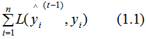
Assuming that the predicted results for the previous t-1 trees are , and the true results are y, with L denoting the loss function, then the current model’s loss function is:
The XGBoost method considers regularization while constructing trees, defining the complexity of each tree as:

Therefore, the loss function including the regularization term is:
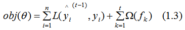
Minimizing (1.3) gives the final objective function:

The objective function, also known as the scoring function, is the standard for measuring the quality of the tree structure. A smaller value indicates a better tree structure. Therefore, the splitting rule for the tree nodes is to choose the point that maximally decreases the value of the tree’s objective function as the splitting point.
As shown in the figure below, the difference in the objective function before and after a node’s split is referred to as Gain.

Choosing the splitting point with the largest Gain leads to the tree’s division, and so on, resulting in a complete tree.
Thus, as long as we know the parameter values in (1.5), we can basically determine the tree model. Among them, denotes the sum of the second derivatives of the loss function for the left child node,
 denotes the sum of the second derivatives of the loss function for the right child node,
 denotes the sum of the first derivatives of the loss function for the left child node,
 denotes the sum of the first derivatives of the loss function for the right child node.
 denotes the regularization coefficient,
 denotes the difficulty of the splitting node,
 and
and define the complexity of the tree. To simplify, once we set the loss function L, the regularization coefficient
  and the difficulty of the splitting nodes
  , we have basically determined the tree model. The key parameters to consider for XGBoost tuning are these three parameters.
1. Regularization
XGBoost considers the regularization term when splitting nodes (as shown in Figure 1.3), reducing overfitting. In fact, XGBoost is also known as “Regularized Boosting” technology.
2. Parallel Processing
Although XGBoost generates each decision tree iteratively, we can achieve parallel processing during node splitting, thus supporting Hadoop implementation.
3. High Flexibility
XGBoost supports custom objective functions and evaluation functions. The evaluation function measures the quality of the model, while the objective function is the loss function. As discussed in the previous section, once we know the loss function, we can determine the splitting rules for nodes by calculating its first and second derivatives.
4. Handling Missing Values
XGBoost has built-in rules for splitting nodes that handle missing values. Users need to provide a unique value (like -999) to represent missing values.
5. Built-in Cross-Validation
XGBoost allows for cross-validation in each iteration, making it easy to obtain cross-validation rates and determine the optimal boosting iteration count without needing traditional grid search methods.
6. Continue from Existing Models
XGBoost can continue training from the results of the previous round, saving runtime, which can be achieved by setting the model parameter “process_type” to update.
XGBoost parameters are divided into three categories:
1. General Parameters: Control the macro functionality of the model.
2. Booster Parameters: Control the tree generation for each iteration.
3. Learning Objective Parameters: Determine the learning scenario, such as the loss function and evaluation function.
3.1 General Parameters
-
booster [default = gbtree]
The available models are gbtree and gblinear. gbtree uses tree-based models for boosting, while gblinear uses linear models. The default is gbtree. Here we only introduce tree boosters, as they outperform linear boosters.
-
silent [default = 0]
When set to 0, it prints running information; when set to 1, it does not print running information.
-
nthread
The number of threads used during XGBoost runtime, defaulting to the maximum number of threads available on the current system.
-
num_pbuffer
The buffer size for prediction data, typically set to the size of the training samples. The buffer retains the prediction results after the last iteration, which is automatically set by the system.
-
num_feature
Sets the feature dimensions to construct the tree model, which is automatically set by the system.
3.2 Booster Parameters
-
eta [default = 0.3]
Controls the weight of the tree model, similar to the learning rate in the AdaBoost algorithm, reducing the weight to avoid overfitting. When optimizing eta, it should be considered in conjunction with the number of iterations (num_boosting_rounding); for instance, if the learning rate is decreased, the maximum number of iterations should be increased; conversely, if the learning rate is increased, the maximum number of iterations should be decreased.
Range: [0,1]
Model iteration formula:
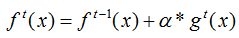
Where denotes the output results of the model combined with the previous t trees,
 denotes the t-th tree model, α represents the learning rate, which controls the weight of model updates.
-
gamma [default = 0]
Controls the minimum loss function value for splitting nodes, corresponding to γ in (1.5). If γ is set too high (making (1.5) less than zero), no node splitting occurs, thus reducing the complexity of the model.
-
lambda [default = 1]
Represents the L2 regularization parameter, corresponding to λ in (1.5). Increasing λ makes the model more conservative, avoiding overfitting.
-
alpha [default = 0]
Represents the L1 regularization parameter. The significance of L1 regularization is that it can reduce dimensionality; increasing the alpha value makes the model more conservative, avoiding overfitting.
Range: [0,∞]
-
max_depth [default=6]
Indicates the maximum depth of the tree. Increasing the depth of the tree raises its complexity, which can easily lead to overfitting. A value of 0 means no limit on the maximum depth of the tree.
Range: [0,∞]
-
min_child_weight [default=1]
Indicates the minimum sum of sample weights for leaf nodes. Unlike the previously mentioned min_child_leaf parameter, min_child_weight refers to the sum of sample weights, while min_child_leaf refers to the total number of samples.
Range: [0,∞]
-
subsample [default=1]
Indicates the random sampling of a certain proportion of samples to construct each tree. Reducing the subsample parameter value makes the algorithm more conservative, avoiding overfitting.
Range: [0,1]
-
colsample_bytree, colsample_bylevel, colsample_bynode
These three parameters indicate random sampling of features and have a cumulative effect.
colsample_bytree indicates the proportion of features used for splitting each tree
colsample_bylevel indicates the proportion of features used for splitting at each level of the tree
colsample_bynode indicates the proportion of features used for splitting at each node of the tree.
For example, if there are 64 features in total and we set {‘colsample_bytree’: 0.5, ‘colsample_bylevel’: 0.5, ‘colsample_bynode’: 0.5}, then 4 features are randomly sampled for splitting at each node of the tree.
Range: [0,1]
-
tree_method string [default = auto]
Indicates the method for constructing the tree, specifically the algorithm for selecting split points, including greedy algorithm, approximate greedy algorithm, and histogram algorithm.
exact: greedy algorithm
approx: approximate greedy algorithm, selecting quantiles for feature splitting
hist: histogram splitting algorithm, which is also used by the LightGBM algorithm.
-
scale_pos_weight [default = 1]
When there is an imbalance between positive and negative samples, setting this parameter to a positive value can speed up algorithm convergence.
Typical values can be set as: (number of negative samples)/(number of positive samples)
-
process_type [default = default]
default: normal boosting tree construction process
update: construct boosting trees from existing models
3.3 Learning Task Parameters
Set parameters based on tasks and objectives
objective, training objective, classification or regression
reg: linear, linear regression
reg: logistic, logistic regression
binary: logistic, using LR for binary classification, outputting probabilities
binary: logitraw, using LR for binary classification, outputting classification scores before logistic transformation.
eval_metric, the metric for evaluating the validation set, defaulting to the objective function settings. By default, mean squared error is used for regression, error rate for classification, and mean average precision for ranking.
rmse: root mean squared error
mae: mean absolute error
error: error rate
logloss: negative log loss
auc: area under the ROC curve
seed [default=0]
The random seed, setting it allows for replicating random data results.
4. Parameter Tuning Example
The original dataset and the dataset processed through feature engineering can be downloaded from the links provided at the beginning. The algorithm is developed in a Jupyter Notebook interactive interface.
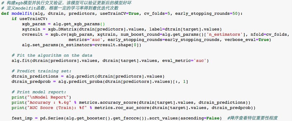
Define the model evaluation function and obtain the optimal iteration count based on a certain learning rate. The function definition is as follows:
Step 1:
Set default parameters based on experience, using the modelfit function to find that the optimal iteration count is 198.

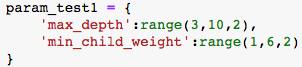
Step 2: Tuning Maximum Tree Depth and Minimum Leaf Node Weight
Based on the optimal iteration count obtained in the first step, update the model parameter n_estimators, then call GridSearchCV from the model_selection class to set up the cross-validation model, and finally call the fit function of the XGBClassifier class to obtain the optimal maximum tree depth and minimum leaf node weight.
a) Set the range for maximum tree depth and minimum leaf node weight:
b) Set up the cross-validation model with GridSearchCV:
c) Update parameters using the fit function of the XGBClassifier class:
Step 3: Tuning the gamma parameter
Step 4: Tuning the subsample and colsample_bytree parameters
Step 5: Tuning the regularization parameters
Steps 3, 4, and 5 follow the same tuning approach as Step 2; further details can be found in the code.
Step 6: Decrease the learning rate and increase the corresponding maximum iteration count. The tuning approach is consistent with Step 1, yielding the optimal iteration count and outputting the cross-validation rate results.
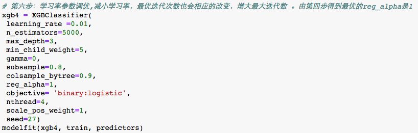
With an iteration count of 2346, the optimal classification result is obtained (as shown in the figure below).
XGBoost is a high-performance learning model algorithm. When you are unsure how to tune the model parameters, you can refer to the steps in the previous section for parameter tuning. In this section, based on the previous content and my project experience, I will share some of my understandings of XGBoost parameter tuning. If there are any errors, please feel free to correct me.
(1) Model Initialization. When initializing model parameters, we try to set the model’s complexity relatively high and then gradually reduce the model complexity through parameter tuning. For example, in the previous section, the initialized parameters were: minimum weight of leaf nodes set to 0, maximum tree depth set to 5, and minimum loss function decrease value set to 0. These parameter initializations all complicate the model.
(2) Learning Rate and Maximum Iteration Count. These two parameters are definitely interrelated. A larger learning rate requires fewer maximum iterations for the same model performance, while a smaller learning rate requires more maximum iterations. XGBoost requires multiple iterations for updating each parameter, so the learning rate and maximum iteration count are the first parameters to consider. The focus of the learning rate and maximum iteration count is not on improving the model’s classification accuracy but on enhancing the model’s generalization ability. Therefore, when the model’s classification accuracy is very high, we should reduce the learning rate in the final step to improve the model’s generalization ability.
(3) Gradually Reducing Model Complexity. The maximum depth of the tree and the minimum weight of leaf nodes are factors that influence model complexity. Based on experience, the tuning order in Section 4 is: maximum tree depth and minimum leaf node weight -> minimum loss function decrease -> row sampling and column sampling -> regularization parameters. In practical projects, I generally follow this order for tuning; if there are different understandings, I welcome discussions.
(4) Feature Engineering: If the model’s accuracy is very low, I suggest not focusing on parameter tuning yet but rather emphasizing features and training data. Features and data determine the upper limit of the model; the model merely approaches this limit.
References:
https://xgboost.readthedocs.io/en/latest/
Recommended Reading
Summary of XGBoost Algorithm Principles
Summary of XGBoost Splitting Point Algorithm