Understanding Word2vec: The Essence of Word Vectors

Summary of Word2vec Reference Materials

Let me briefly describe my deep dive into Word2vec: I first looked at Mikolov’s two original papers on Word2vec, but found myself still confused after reading them. The main reason is that these papers omit too much theoretical background and derivation details. I then revisited Bengio’s 2003 JMLR paper and Ronan’s 2011 JMLR paper, which gave me some understanding of topic models and using CNN for NLP tasks, but I still couldn’t fully grasp Word2vec. At this point, I started reading a lot of Chinese and English blogs, and I was particularly drawn to a blog by 北漂浪子 that had a high readership, which systematically explained the ins and outs of Word2vec. The most valuable part was the in-depth analysis of the implementation details of the code. After reading it, I understood many details but still felt some fog. Finally, I saw a recommendation for Xin Rong’s English paper on Quora, and after reading it, I felt enlightened and exhilarated; it became my top recommendation for Word2vec reference materials. Below I will list all the Word2vec related reference materials I have read and provide evaluations.

1. Mikolov’s two original papers:

• “Efficient estimation of word representations in vector space”

• This paper discusses two tricks used in training Word2vec: hierarchical softmax and negative sampling.

• “Distributed Representations of Sentences and Documents”

• This paper proposes a more streamlined language model framework based on previous work and is used to generate word vectors; this framework is Word2vec.

1. Advantages: The pioneering work of Word2vec, both papers are worth reading.

2. Disadvantages: They see the trees but not the forest and leaves; after reading, one does not grasp the essence. Here, ‘forest’ refers to the theoretical foundation of the Word2vec model—i.e., the language model represented in the form of a neural network, while ‘leaves’ refer to specific neural network forms, theoretical derivations, implementation details of hierarchical softmax, etc.

北漂浪子’s blog: “Deep Learning Word2vec Notes – Basics”

• Advantages: Very systematic, combined with source code analysis, and written in plain language.

• Disadvantages: Too verbose, a bit hard to grasp the essence.

Yoav Goldberg’s paper: “Word2vec Explained – Deriving Mikolov et al.’s Negative-Sampling Word-Embedding Method”

• Advantages: The derivation of the negative-sampling formula is very comprehensive.

• Disadvantages: Not comprehensive enough, and mostly formulas without illustrations, somewhat dry.

Xin Rong’s paper: “Word2vec Parameter Learning Explained”:

• Highly Recommended!

• The theory is complete and easy to understand, hitting the nail on the head, with both high-level intuition explanations and detailed derivation processes.

• You must read this paper! You must read this paper! You must read this paper!

Laiswei’s doctoral dissertation “Research on Semantic Vector Representation Methods for Words and Documents Based on Neural Networks” and his blog (nickname: licstar)

• This can serve as a more in-depth and comprehensive reading, which not only covers Word2vec but also reviews all mainstream methods of word embedding.

Several experts’ answers on Zhihu: “What are the advantages of Word2vec compared to previous word embedding methods?”

• Famous scholars like Liu Zhiyuan, Qiu Xipeng, and Li Shaohua express their views on Word2vec from different angles; it is worth a look.

Sebastian’s blog: “On Word Embeddings – Part 2: Approximating the Softmax”

• This blog explains the approximation methods of softmax in detail; Word2vec’s hierarchical softmax is just one of them.

What is Word2vec?

Before discussing Word2vec, let’s talk about NLP (Natural Language Processing). In NLP, the finest granularity is words, words form sentences, sentences form paragraphs, chapters, and documents. Therefore, to address problems in NLP, we first need to tackle words.

For example, to determine the part of speech of a word, whether it is a verb or a noun. Using a machine learning approach, we have a series of samples (x, y), where x is the word, and y is its part of speech. We want to build a mapping f(x) -> y, but here the mathematical model f (such as a neural network, SVM) only accepts numerical input, while words in NLP are human abstractions and are in symbolic form (such as Chinese, English, Latin, etc.), so we need to convert them into numerical form, or in other words—embed them into a mathematical space. This embedding method is called word embedding, and Word2vec is one such word embedding.

In my previous work “It’s All a Routine: Understanding Time Series and Data Mining from God’s Perspective”, I mentioned that most machine learning models can be summarized as:

f(x) -> y

In NLP, treating x as a word in a sentence, y is the context words of that word, then f is a model often seen in NLP called “topic model”. The purpose of this model is to determine whether the sample (x, y) conforms to the laws of natural language; in simpler terms, it means: does word x and word y together make sense?

Word2vec stems from this idea, but its ultimate goal is not to train f to perfection, but rather to focus on the byproduct after training the model—the model parameters (specifically, the weights of the neural network) and use these parameters as a certain vector representation of input x, which is called the word vector (it’s okay if you don’t understand this part, we will analyze it in detail in the next section).

Let’s look at an example of how to use Word2vec to find similar words:

• For the sentence: “They praise Wu Yanzu for being handsome to the point of having no friends”, if the input x is “Wu Yanzu”, then y can be words like “they”, “praise”, “handsome”, “no friends”.

• In another sentence: “They praise me for being handsome to the point of having no friends”, if the input x is “me”, it’s easy to see that the context y is the same as in the previous sentence.

• Thus, f(Wu Yanzu) = f(me) = y, so big data tells us: I = Wu Yanzu (a perfect conclusion).

Word2vec is an effective way to create word embeddings, existing since 2013. But beyond being a method for word embeddings, some of its concepts have been proven effective in creating recommendation engines and understanding time series data in commercial, non-language tasks. Companies like Airbnb, Alibaba, and Spotify have drawn inspiration from the NLP field and applied it to their products, thus supporting new types of recommendation engines.

In this article, we will discuss the concept of embeddings and the mechanism of generating embeddings using Word2vec. Let’s start with an example to familiarize ourselves with using vectors to represent things. Did you know that your personality can be represented by just a list of five numbers (vectors)?

Personality Embedding: What Kind of Person Are You?

How can we represent how introverted/extroverted you are on a scale from 0 to 100 (where 0 is the most introverted and 100 is the most extroverted)? Have you ever taken a personality test like MBTI or the Big Five personality traits test? If you haven’t, these tests will ask you a series of questions and then score you on many dimensions, one of which is introversion/extroversion.

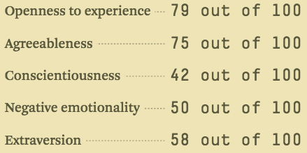
Example of the five-factor personality traits test results. It can really tell you a lot about yourself and has predictive power in academic, personality, and career success. You can find the test results here.

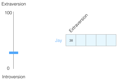
Assuming my introversion/extroversion score is 38/100. We can visualize it this way:

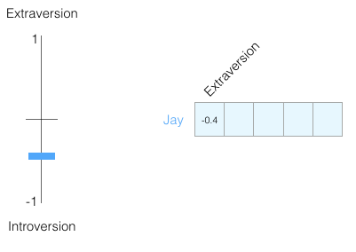
Let’s narrow the range down to -1 to 1:

When you only know this one piece of information, how much do you think you understand about this person? Not much. People are complex, so let’s add another test score as a new dimension.

We can represent the two dimensions as a point on a graph or as a vector from the origin to that point. We have great tools to handle the upcoming vectors.

I have hidden the personality traits we are plotting so that you will gradually get used to extracting valuable information from a vector representation of a personality without knowing what each dimension represents.

We can now say this vector partially represents my personality. This representation becomes useful when you want to compare two other people to me. Suppose I was hit by a bus, and I need to be replaced by a personality similar to mine; which of the two people in the graph is more like me?

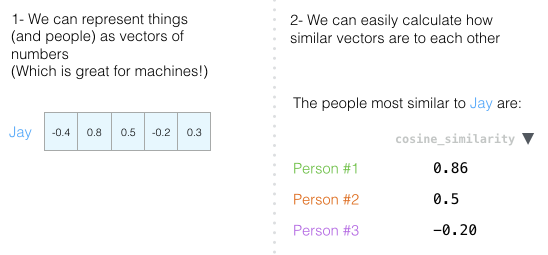
When dealing with vectors, a common way to compute similarity scores is cosine similarity:

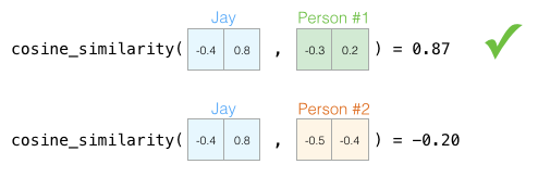
Person 1 is more similar to me in personality. Vectors pointing in the same direction (length also matters) have higher cosine similarity.

Once again, two dimensions are still insufficient to capture enough information about different populations. Psychology has identified five major personality traits (along with numerous sub-traits), so let’s use all five dimensions for comparison:

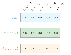
The problem with using five dimensions is that we can no longer neatly draw small arrows on a two-dimensional plane. This is a common problem in machine learning, where we often need to think in higher-dimensional spaces. But fortunately, cosine similarity still works; it applies to any number of dimensions:

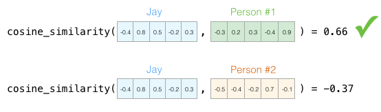
Cosine similarity applies to any number of dimensions. These scores are better than the previous ones because they are calculated based on higher-dimensional comparisons.

At the end of this section, I would like to propose two central ideas:

1. We can represent people and things as algebraic vectors (which is great for machines!).

2. We can easily calculate relationships between similar vectors.

Word Embedding

With the understanding from the previous text, let’s continue to look at examples of trained word vectors (also known as word embeddings) and explore some of their interesting properties.

This is a word embedding for the word “king” (GloVe vectors trained on Wikipedia):

[ 0.50451 , 0.68607 , -0.59517 , -0.022801, 0.60046 , -0.13498 , -0.08813 , 0.47377 , -0.61798 , -0.31012 , -0.076666, 1.493 , -0.034189, -0.98173 , 0.68229 , 0.81722 , -0.51874 , -0.31503 , -0.55809 , 0.66421 , 0.1961 , -0.13495 , -0.11476 , -0.30344 , 0.41177 , -2.223 , -1.0756 , -1.0783 , -0.34354 , 0.33505 , 1.9927 , -0.04234 , -0.64319 , 0.71125 , 0.49159 , 0.16754 , 0.34344 , -0.25663 , -0.8523 , 0.1661 , 0.40102 , 1.1685 , -1.0137 , -0.21585 , -0.15155 , 0.78321 , -0.91241 , -1.6106 , -0.64426 , -0.51042 ]

This is a list of 50 numbers. By observing the values, we can’t tell much, but let’s visualize it a bit to compare with other word vectors. We will line up all these numbers:

Let’s color-code the cells based on their values (red for values close to 2, white for values close to 0, and blue for values close to -2):

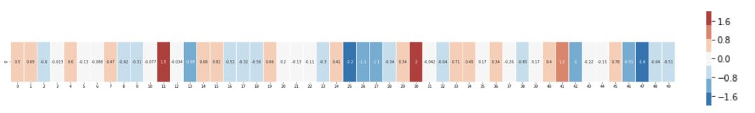
We will ignore the numbers and just look at the colors to indicate the values of the cells. Now let’s compare “king” with other words:

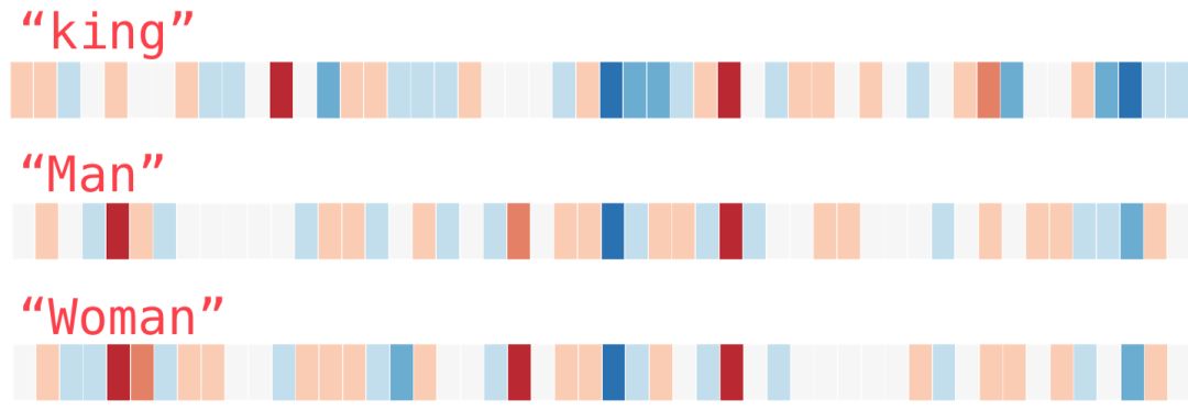
Notice how “Man” and “Woman” are more similar to each other than either is to “King”? This suggests something. These vector visualizations nicely showcase the information/meaning/associations of these words.

This is another example list (look for similar colors by scanning the columns vertically):

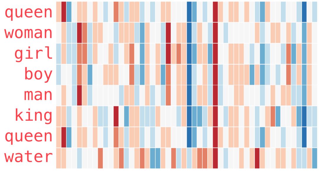
There are several points to note:

1. All these different words have a straight red column. They are similar in this dimension (even though we don’t know what each dimension represents).

2. You can see that “woman” and “girl” are similar in many respects, and so are “man” and “boy”.

3. “Boy” and “girl” also have similarities, but those differ from those with “woman” or “man”. Can these be summarized into a vague concept of “youth”? Perhaps.

4. Except for the last word, all words represent people. I added an object “water” to show the differences between categories. You can see the blue column goes down and stops before the word embedding for “water”.

5. “King” and “queen” are similar to each other but different from all other words. Can these be summarized into a vague concept of “royalty”? Perhaps.

Analogy

A famous example that showcases the wonderful properties of embeddings is analogy. We can add and subtract word embeddings and get interesting results. A well-known example is the formula: “king” – “man” + “woman”:

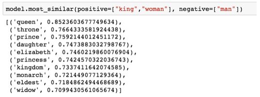
Using the Gensim library in Python, we can add and subtract word vectors, and it will find the words most similar to the resulting vector. This image shows the list of most similar words, each with cosine similarity.

We can visualize this analogy as before:

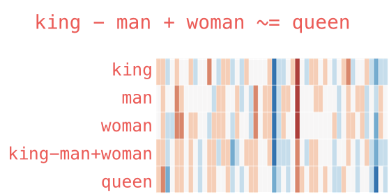
The vector generated from “king” – “man” + “woman” is not exactly equal to “queen”, but “queen” is the closest word to it among the 400,000 word embeddings included in this set.

Now that we have seen trained word embeddings, let’s learn more about the training process. But before we begin using Word2vec, we need to look at the parent concept of word embeddings: neural language models.

Language Models

If we were to cite the most typical example of natural language processing, it would be the next-word prediction feature in smartphone input methods. This is a feature used hundreds of times daily by billions of people.

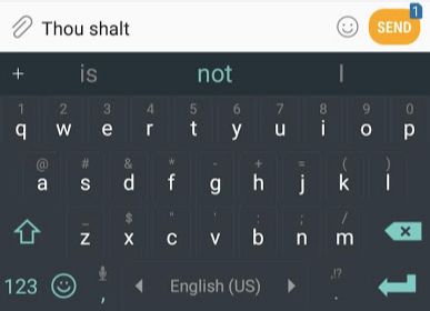
Next-word prediction is a task that can be achieved through language models. Language models try to predict the next word that may follow a list of words (for example, two words).

In the mobile screenshot above, we can think of the model receiving two green words (thou shalt) and recommending a set of words (“not” is among the most likely to be chosen):

We can imagine this model as this black box:

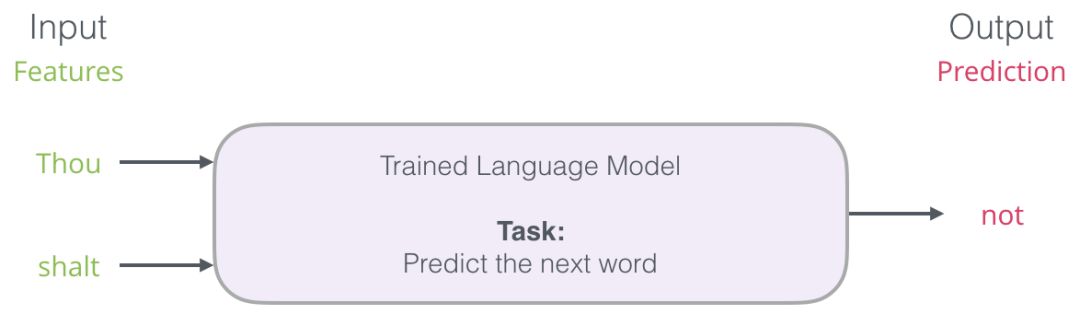
But in fact, the model does not output just one word. Instead, it scores all the words it knows (the model’s vocabulary, which can range from a few thousand to millions of words) by probability, and the input method program selects the highest-scoring one to recommend to the user.

The output of the natural language model is the probability scores of the words known by the model; we usually express probabilities as percentages, but in fact, a score like 40% is represented as 0.4 in the output vector group.

The natural language model (see Bengio 2003) completes predictions in three steps after training:

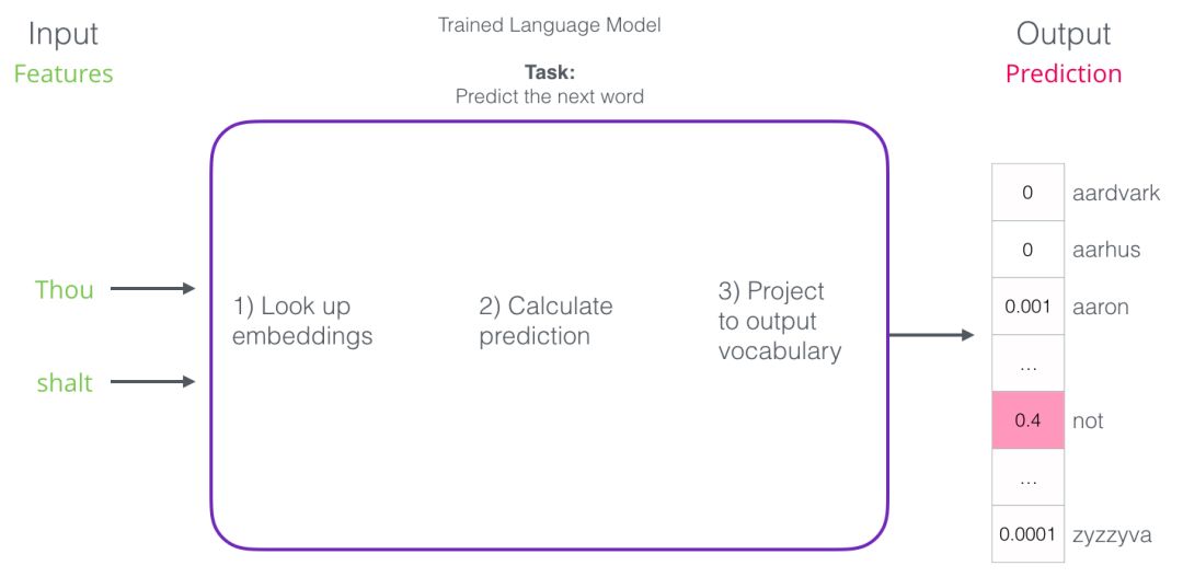
The first step is the most relevant to us because we are discussing Embedding. After training, the model generates a matrix mapping all words in the vocabulary. During prediction, our algorithm queries the input word in this mapping matrix and calculates the predicted value:

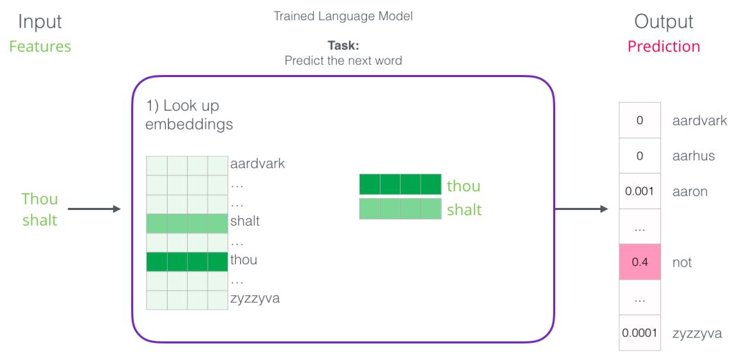
Now let’s focus on model training to learn how to construct this mapping matrix.

Language Model Training

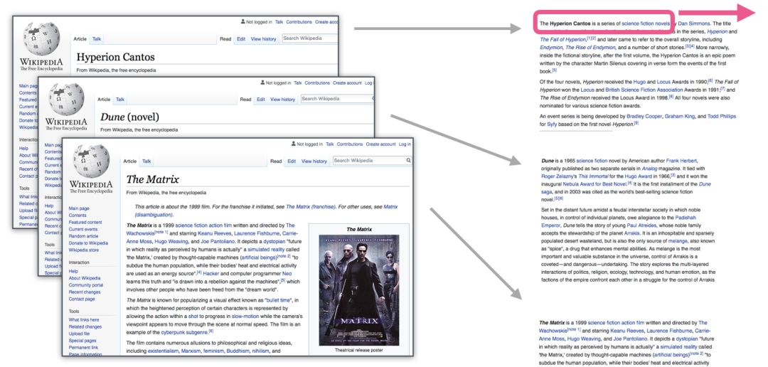
Compared to most other machine learning models, language models have a significant advantage: we have rich text to train the language model. All our books, articles, Wikipedia, and various types of textual content are available. In contrast, many other machine learning model developments require manually designed data or specially collected data.

We can obtain their mapping relationships by finding words that frequently appear near each word. The mechanism is as follows:

1. First, acquire a large amount of text data (for example, all Wikipedia content).

2. Then we establish a sliding window that can move along the text (for example, a window containing three words).

3. Using this sliding window, we can generate a large amount of sample data for training the model.

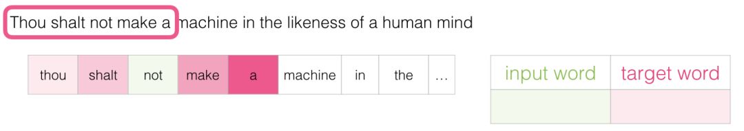
As this window slides along the text, we can (in reality) generate a dataset for model training. To clarify this process, let’s see how the sliding window processes this phrase:

At the beginning, the window locks onto the first three words of the sentence:

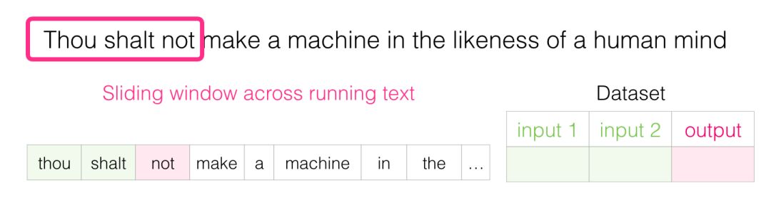
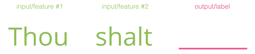
We treat the first two words as features and the third word as the label:

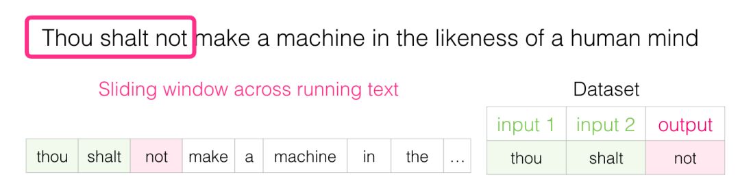
This generates the first sample in the dataset, which will be used in our subsequent language model training.

Next, we slide the window to the next position and generate the second sample:

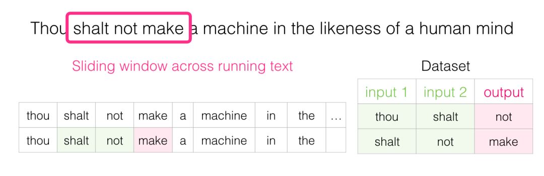
The second sample is also generated.

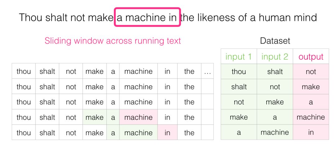
Before long, we can obtain a large dataset, from which we can see which words tend to appear after different word groups:

In practice, the model is often trained as we slide the window. However, I think separating the dataset generation and model training into two phases makes it clearer and easier to understand. Besides using neural networks for modeling, a technique called N-grams is often used for model training.

If you want to understand the transition from using N-grams models to neural models in real products, you can check out a blog published by Swiftkey (my favorite Android input method) in 2015, which discusses their natural language model and compares it with early N-grams models. I like this example because it tells you how to clearly explain the attributes of the Embedding algorithm in marketing presentations.

Considering Both Ends

Fill in the blanks based on the previous information:

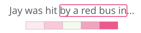
In front of the blank, the background I provided is five words (if ‘bus’ is mentioned beforehand), most people would definitely fill in ‘bus’ in the blank. But if I give you another piece of information—such as a word after the blank, will the answer change?

Now the content filled in the blank has completely changed. At this point, the word ‘red’ is most likely to fit in that position. From this example, we learn that both the preceding and following words carry informational value. It turns out we need to consider the words in both directions (the left and right words of the target word). So how do we adjust the training method to meet this requirement? Let’s continue to read.

Skipgram Model

We need to consider not just the previous two words of the target word but also the two words that come after it.

If we do this, the model we are actually building and training will look like this:

This architecture is called Continuous Bag of Words (CBOW), as discussed in a paper on Word2vec.

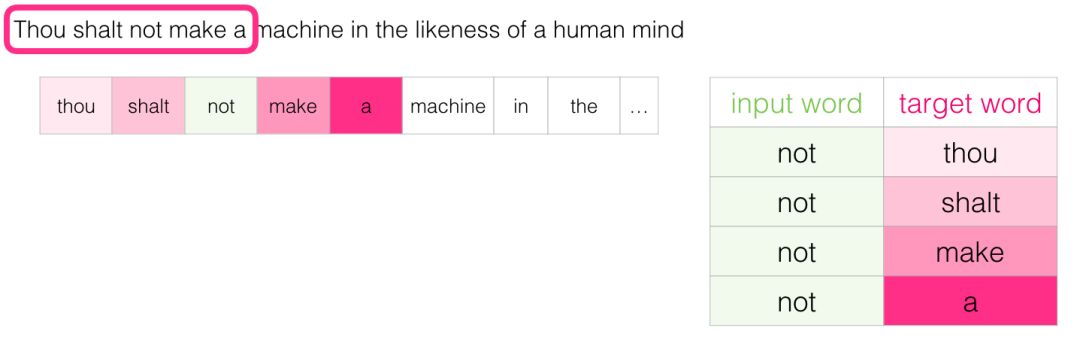
There is another architecture that does not guess the target word based on the surrounding context (previous and following words) but rather predicts the possible surrounding words based on the current word. Let’s imagine the sliding window in training data as shown below:

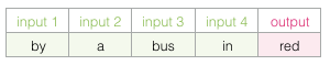
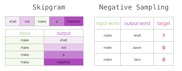
The words in the green box are the input words, while the pink box contains the possible output results.

The depth of the pink box color indicates the number of independent samples generated by the sliding window:

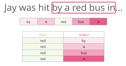
This method is called the Skipgram architecture. We can visualize the content of the sliding window as follows.

This provides four samples for the dataset:

Then we move the sliding window to the next position:

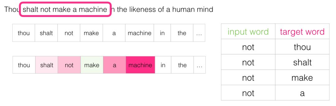
This generates another four samples:

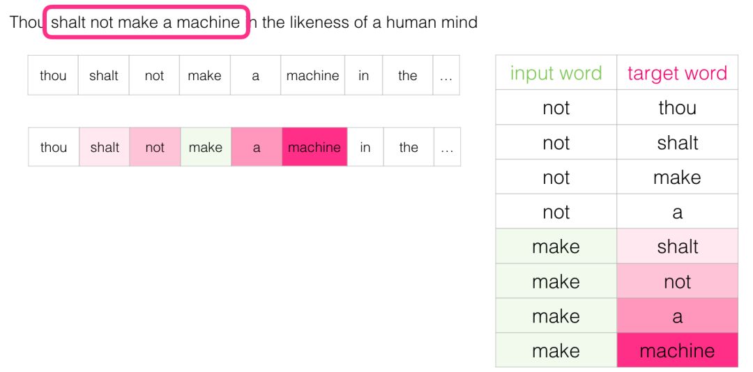
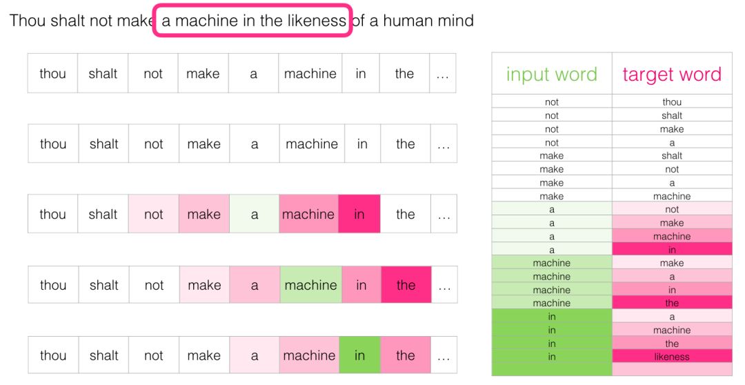
After moving a few positions, we can obtain a batch of samples:

Revisiting the Training Process

Now that we have obtained the training dataset for the Skipgram model from existing text, let’s see how to use it to train a natural language model that predicts adjacent vocabulary.

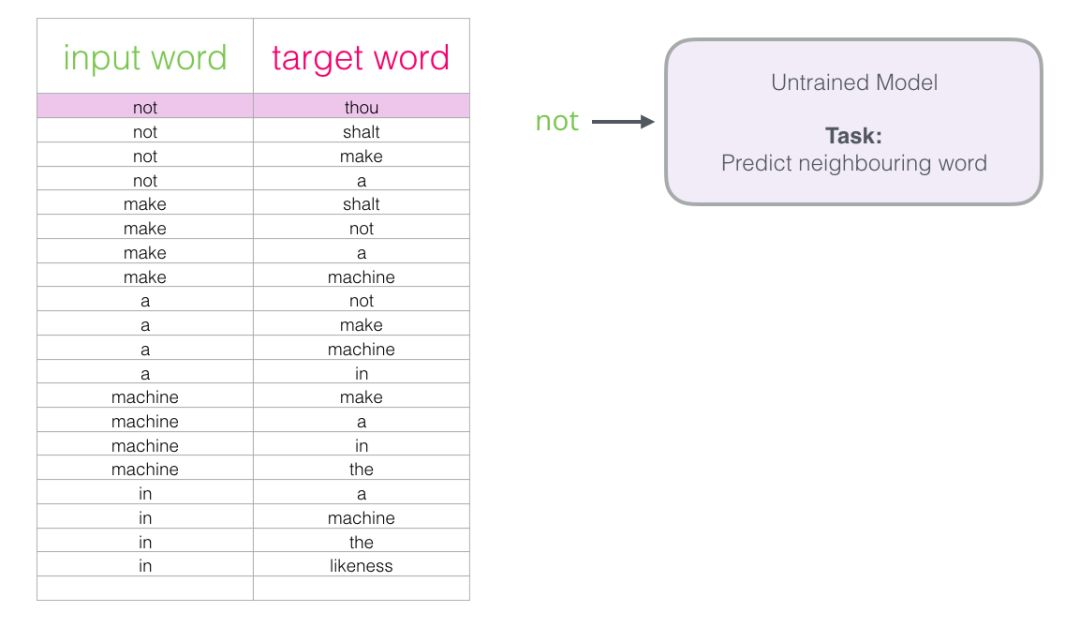
Starting with the first sample in the dataset, we input the features into an untrained model and let it predict a possible adjacent word.

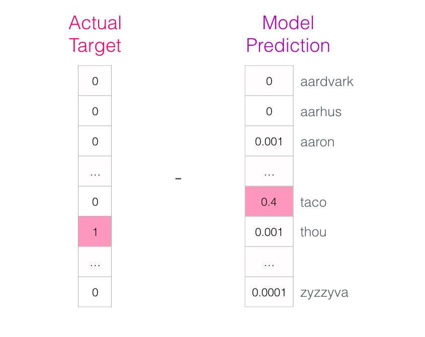
The model will perform three steps and output a prediction vector (corresponding to the probability of each word in the vocabulary). Since the model is untrained, the predictions at this stage will definitely be incorrect. But that’s okay; we know which word we should guess—the word is the output label in our training dataset:

The target word’s probability is 1, and the probabilities of all other words are 0, so the vector formed by these values is the “target vector”.

How big is the model’s bias? By subtracting the two vectors, we can obtain the bias vector:

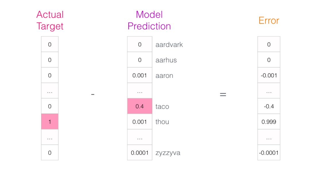
This error vector can now be used to update the model, so in the next round of predictions, if we input “not”, we are more likely to get “thou” as the output.

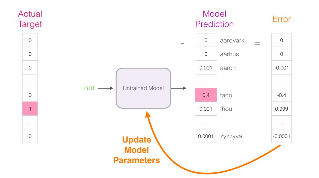
This is actually the first step of training. Next, we continue to perform the same operation on the next sample in the dataset until we go through all the samples. This is one epoch. We repeat this for several epochs to obtain a trained model, and then we can extract the embedding matrix from it for other applications.

This certainly helps us understand the entire process, but this is still not the actual training method of Word2vec. We missed some key ideas.

Negative Sampling

Recall the three steps that the neural language model uses to calculate prediction values:

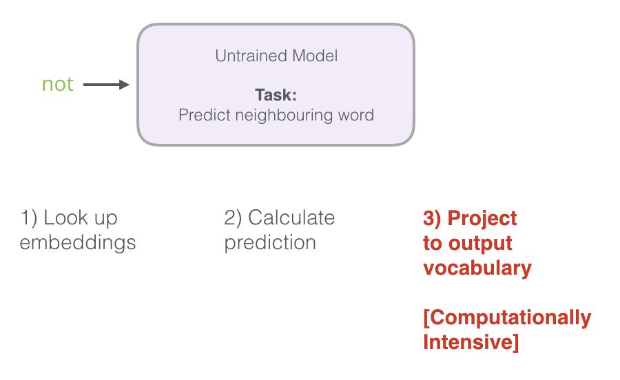
From a computational perspective, the third step is very costly—especially when we need to do it for every training sample in the dataset (easily reaching tens of millions). We need to find ways to improve performance.

One approach is to divide the target into two steps:

1. Generate high-quality word embeddings (don’t worry about predicting the next word).

2. Use these high-quality embeddings to train the language model (perform next-word prediction).

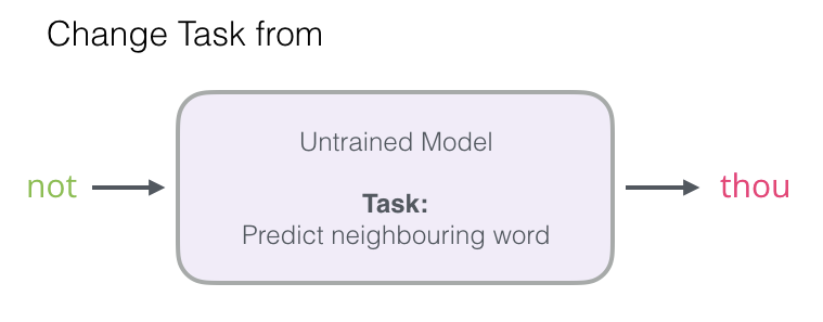
In this article, we will focus on the first step (because this article focuses on embeddings). To generate high-quality embeddings using a high-performance model, we can change the task of predicting adjacent words:

Switch it to a model that extracts input and output words and outputs a score indicating whether they are neighbors (0 means “not neighbors”, 1 means “neighbors”).

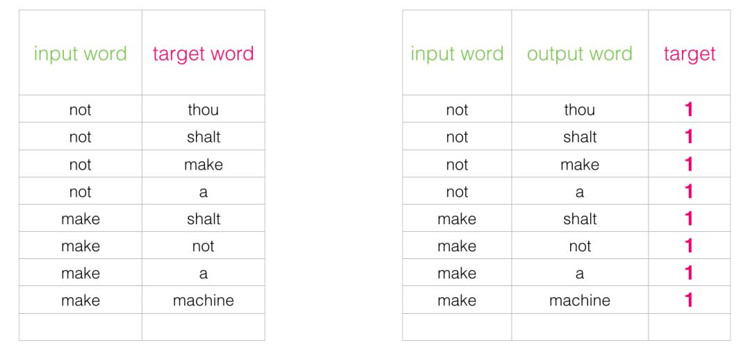
This simple transformation changes the required model from a neural network to a logistic regression model—making it simpler and faster to compute.

This switch requires us to change the structure of the dataset—the label values now include a new column with values of 0 or 1. They will all be 1 because all the words we add are neighbors.

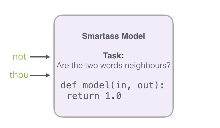
Now the computation speed is astonishing—able to process millions of examples in just minutes. However, we still need to address a loophole. If all examples are neighbors (target: 1), our “genius model” may be trained to always return 1—accuracy is 100%, but it learns nothing and will only produce garbage embedding results.

To solve this problem, we need to introduce negative samples into the dataset—samples of words that are not neighbors. Our model needs to return 0 for these samples. The model must work hard to solve this challenge—while still maintaining high speed.

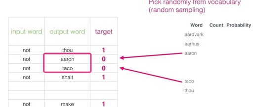
For each sample in our dataset, we add negative examples. They have the same input word, with labels of 0.

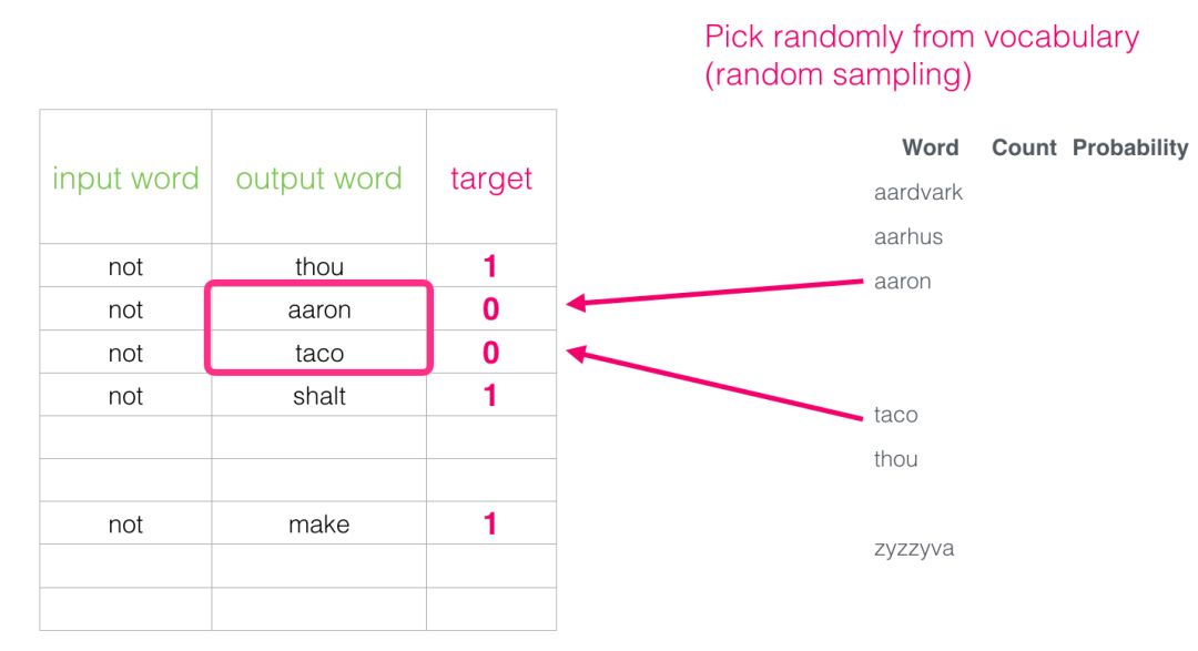
But what do we fill in as output words? We randomly draw words from the vocabulary.

This idea is inspired by noise contrastive estimation. We compare the actual signal (positive examples of adjacent words) with noise (randomly chosen non-neighbors). This leads to a significant trade-off in computational and statistical efficiency.

Noise Contrastive Estimation

http://proceedings.mlr.press/v9/gutmann10a/gutmann10a.pdf

Skipgram with Negative Sampling (SGNS)

We have now introduced two (pairs of) core ideas in Word2vec: negative sampling and skipgram.

Word2vec Training Process

Now that we understand the two central ideas of skipgram and negative sampling, we can continue to closely study the actual training process of Word2vec.

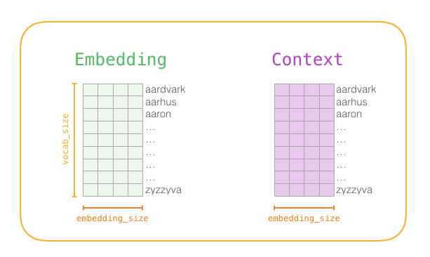
Before the training process begins, we preprocess the text we are training the model on. In this step, we determine the size of the vocabulary (which we call vocab_size, e.g., 10,000) and which words it contains.

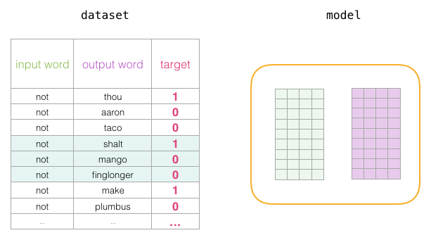
At the start of the training phase, we create two matrices—the Embedding matrix and the Context matrix. These two matrices embed each word in our vocabulary (so vocab_size is one of their dimensions). The second dimension is the length of the embeddings we want each time (embedding_size—300 is a common value, but we have also seen examples of 50).

At the start of the training process, we initialize these matrices with random values. Then we begin the training process. In each training step, we take an adjacent example and its related non-adjacent examples. Let’s look at our first set:

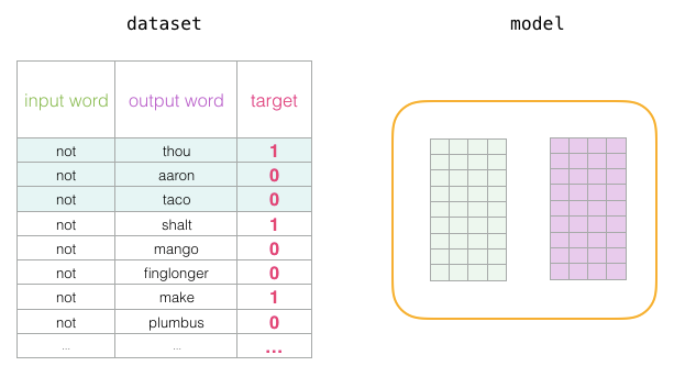
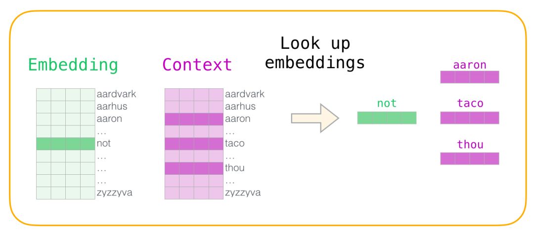
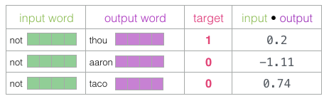
Now we have four words: the input word “not” and the output/context word: “thou” (the actual neighbor word), “aaron” and “taco” (negative examples). We continue to look for their embeddings— for the input word, we check the Embedding matrix. For the context words, we check the Context matrix (even though both matrices embed each word in our vocabulary).

Then, we calculate the dot product of the input embedding with each context embedding. In each case, the result will be a number representing the similarity between the input and context embeddings.

Now we need a way to convert these scores into something that looks like probabilities—we need them all to be positive and between 0 and 1. The sigmoid function is perfect for this task.

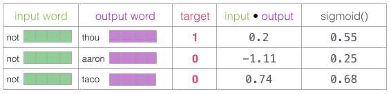
Now we can view the output of the sigmoid operation as the model’s output for these examples. You can see that “taco” scores the highest, and “aaron” the lowest, both before and after the sigmoid operation.

Since the untrained model has made predictions, and we indeed have real target labels for comparison, let’s compute the error in the model’s predictions. To do this, we simply subtract the sigmoid scores from the target labels.

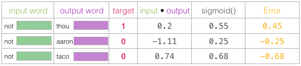
error = target – sigmoid_scores

This is the “learning” part of “machine learning”. Now we can use this error score to adjust the embeddings for “not”, “thou”, “aaron”, and “taco” so that when we make this calculation next time, the results will be closer to the target scores.

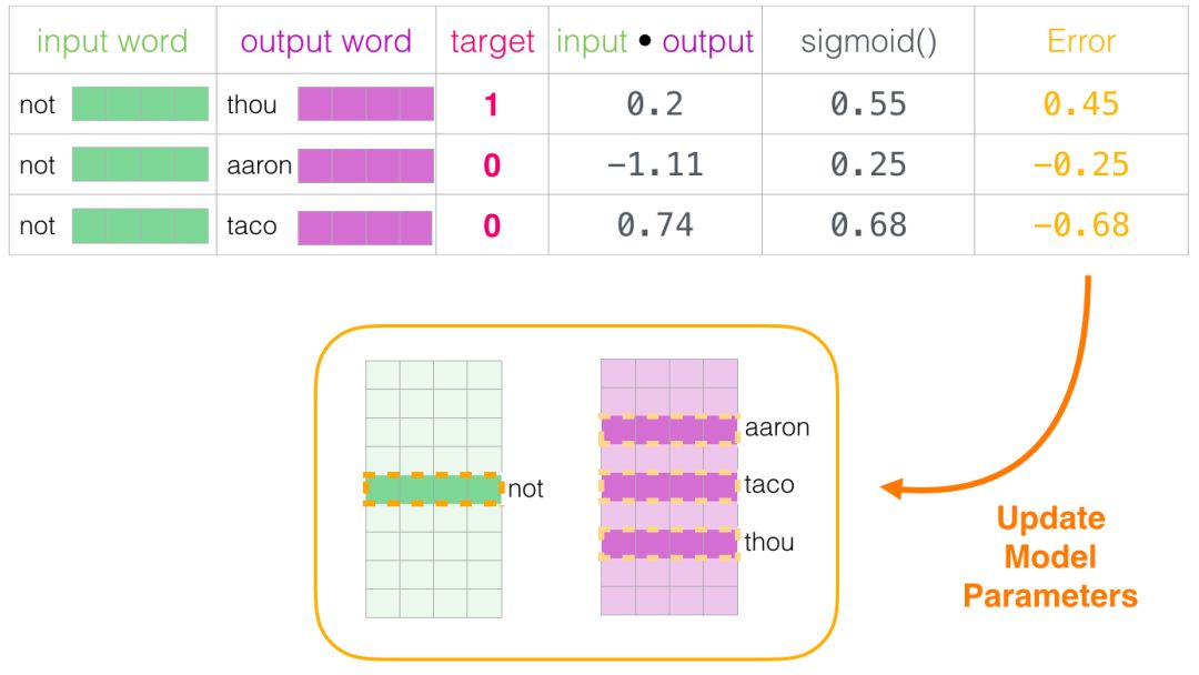
The training step ends here. We have obtained better embeddings for the words used in this step (“not”, “thou”, “aaron”, and “taco”). We now proceed to the next step (the next adjacent sample and its related non-adjacent samples) and repeat the same process.

As we loop through the entire dataset multiple times, the embeddings will continue to improve. Then we can stop the training process, discard the Context matrix, and use the Embeddings matrix as the trained embeddings for the next task.

Window Size and Number of Negative Samples

Two key hyperparameters in the training process of Word2vec are window size and the number of negative samples.

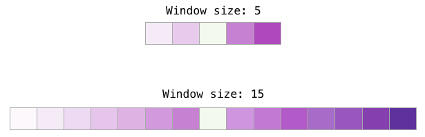
Different tasks suit different window sizes. A heuristic approach is that using a smaller window size (2-15) yields embeddings where a high similarity score between two embeddings indicates that these words are interchangeable (note that if we only look at words that are very close together, antonyms can often be interchangeable—for example, good and bad often appear in similar contexts). Using a larger window size (15-50 or even more) will yield embeddings where similarity better indicates word relevance. In practice, you usually need to guide the embedding process to help readers get a similar “sense”. Gensim defaults to a window size of 5 (including two words before and after the input word, in addition to the input word itself).

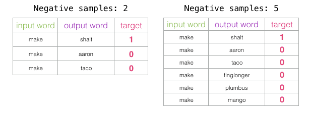The number of negative samples is another factor in the training process. The original paper suggests that 5-20 negative samples is an ideal number. It also notes that when you have a sufficiently large dataset, 2-5 seems to be enough. Gensim defaults to 5 negative samples.

Conclusion

I hope you now have an understanding of word embeddings and the Word2vec algorithm. I also hope that now when you read a paper that mentions “skipgram with negative sampling” (SGNS), you have a better grasp of these concepts.

Machine Learning Algorithms AI Big Data Technology

Search public account to add: datanlp

Long press the image to identify the QR code

People who have read this article also viewed the following articles:

TensorFlow 2.0 Deep Learning Case Practice

Using MaskRCNN for Table Detection Based on the 400,000 Table Dataset TableBank

PDF of Natural Language Processing Based on Deep Learning (Chinese/English)

Deep Learning Chinese Version First Edition – Zhou Zhihua Team

[Complete Video Course] The Most Comprehensive Series of Target Detection Algorithm Explanations, Easy to Understand!

“Meituan Machine Learning Practice”_ Meituan Algorithm Team.pdf

“Deep Learning Introduction: Theory and Implementation Based on Python” High Definition Chinese PDF + Source Code

“Deep Learning: Practice Based on Keras” PDF and Code

Feature Extraction and Image Processing (Second Edition).pdf

Python Employment Class Learning Video, From Entry to Practical Projects

Latest 2019 “PyTorch Natural Language Processing” English and Chinese PDF + Source Code

“21 Projects to Master Deep Learning: Detailed Explanation Based on TensorFlow” Complete PDF with Attached Book Code

“Deep Learning with PyTorch” PDF with Attached Book Source Code

PyTorch Deep Learning Quick Practice Entry “pytorch-handbook”

[Download] Douban Rating 8.1, “Machine Learning in Action: Based on Scikit-Learn and TensorFlow”

“Python Data Analysis and Mining Practice” PDF + Complete Source Code

Complete Knowledge Graph Project Practice Video in the Automotive Industry (All 23 Lessons)

Li Mu’s Open Source “Hands-on Learning Deep Learning”, Berkeley Deep Learning (Spring 2019) Textbook

Notes and Code are Clear and Understandable! Li Hang’s “Statistical Learning Methods” Latest Resource Set!

“Neural Networks and Deep Learning” Latest 2018 Edition Chinese and English PDF + Source Code

Deploy Machine Learning Models as REST APIs

FashionAI Clothing Attribute Tag Image Recognition Top 1-5 Solutions Sharing

Important Open Source! CNN-RNN-CTC Implementation of Handwritten Chinese Character Recognition

YOLO3 Detecting Irregular Chinese Characters in Images

As a Machine Learning Algorithm Engineer, why can’t you pass the interview?

Qianhai Credit Big Data Algorithm: Risk Probability Prediction

[Keras] Complete Implementation of ‘Traffic Sign’ Classification and ‘Receipt’ Classification Projects, Allowing You to Master Deep Learning Image Classification

VGG16 Transfer Learning, Implementing Medical Image Recognition Classification Project

Feature Engineering (Part One)

Feature Engineering (Part Two): Expansion, Filtering, and Chunking of Text Data

Feature Engineering (Part Three): Feature Scaling, From Bag of Words to TF-IDF

Feature Engineering (Part Four): Categorical Features

Feature Engineering (Part Five): PCA Dimensionality Reduction

Feature Engineering (Part Six): Non-linear Feature Extraction and Model Stacking

Feature Engineering (Part Seven): Image Feature Extraction and Deep Learning

How to Use the New Decision Tree Ensemble Cascade Structure gcForest for Feature Engineering and Scoring?

Machine Learning Yearning Chinese Translation Manuscript

Ant Financial 2018 Autumn Recruitment – Algorithm Engineer (Four Interviews) Passed

Global AI Challenge – Scene Classification Competition Source Code (Multi-model Fusion)

Stanford CS230 Official Guide: CNN, RNN, and Tips Quick Reference (Print and Collect)

Python + Flask Build CNN Online Recognition Handwritten Chinese Website

Chinese Academy of Sciences Kaggle Global Text Matching Competition Chinese Team No. 1 – Deep Learning and Feature Engineering

Continuously Updated Resources

Deep Learning, Machine Learning, Data Analysis, Python

Search public account to add: datayx