
Source: Submission Author: Aksy
Editor: Senior Sister
Video Link: https://ai.deepshare.net/detail/p_5ee62f90022ee_zFpnlHXA/6
5. Comparison of Models (Model Architectures Section of the Paper)
Before the introduction of word2vec, NNLM and RNNLM trained word vectors by training language models using statistical methods.
This section mainly compares the following three models:
-
Feedforward Neural Net Language Model -
Recurrent Neural Net Language Model -
Parallel Training of Neural Networks
5.1 Feedforward Neural Network Language Model (NNLM)
5.1.1 Feedforward Neural Net Language Model
The full name of the feedforward neural network language model is Feedforward Neural Net Language Model, abbreviated as NNLM, also known as deep neural network or fully connected neural network.
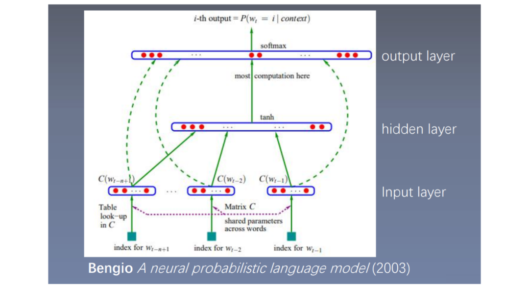
Reference: Bengio A neural probabilistic language model (2003)
In NLP tasks, the first step is to construct word2id and id2word, both of which are dictionary types; the key of word2id is the word and the value is the id, while id2word does the opposite, indicating that each word corresponds to an id.
-
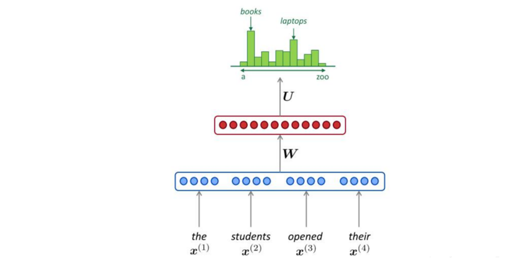
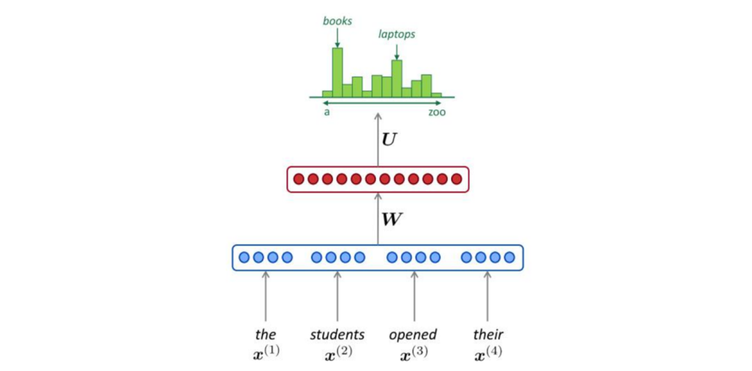
Input Layer: The input is an index, which represents the word’s number, putting all words together to form a dictionary, so each word has a number representing its position. Each index is mapped to a vector, and these vectors are concatenated (concat). For example, if the input consists of n-1 words, and each word is 100-dimensional, then after concatenation, it becomes 100×(n-1) dimensional; -
Hidden Layer: The resulting 100×(n-1) dimensional vector from the previous step is input into a fully connected layer, using the tanh activation function; -
Output Layer: The result from the previous step connects to another fully connected layer, followed by softmax.
Based on the previous n-1 words, it predicts the probability of the nth word, which is the n-gram model. The input goes to the network input layer, is mapped to vectors, concatenated, and after passing through two fully connected layers, softmax predicts the probability of the nth word, thus obtaining the probabilities of each word in the sentence, and consequently the probability of the sentence.
The advantage of the language model is that it is an unsupervised model, requiring no labeled corpus; relevant sentences can be crawled from websites. It predicts the nth word using the previous n-1 words in an unsupervised manner.
To construct the model, padding is first applied before a sentence to predict the first word, generating the corpus where the previous n-1 words serve as features and the next word as the label, and so on, to construct the dataset required for training the feedforward neural network. The model is then optimized using gradient descent to maximize the probability of the correct word output.
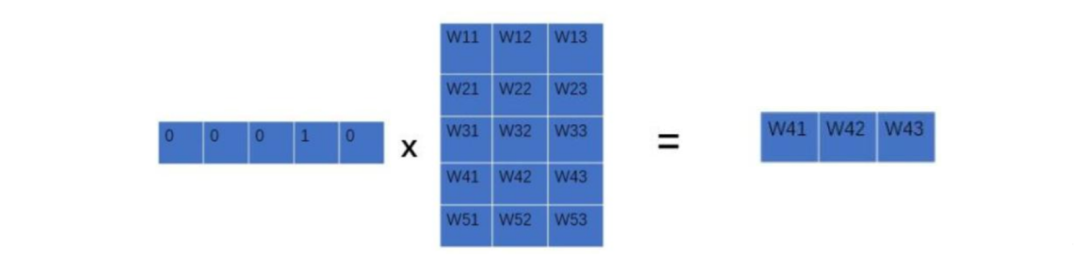
Input Layer: The words (index) are mapped to vectors, equivalent to a 1×V one-hot vector multiplied by a V×D vector to obtain a 1×D vector, where the V×D vector represents a word vector for each row.
Parallel Computation:
Hidden Layer: A fully connected layer with a tanh activation function.
Where represents the bias, is a parameter, and represents parameters similar to and.
Output Layer: A fully connected layer followed by a softmax function to generate a probability distribution.
Where is a vector:
5.1.2 Relationship Between Language Model Perplexity and Loss
How to calculate perplexity?
It requires predicting the probability of each word in each sentence and multiplying them together. This approach is feasible, but there are more convenient and clever methods in practice.
First write the Loss to ensure that the predicted probability of each correct word is maximized, using the cross-entropy loss function; this Loss is for a single sentence:
Where represents the number of words in the sentence. Perplexity is the probability of the sentence raised to the power of -1/T.
Thus, given the loss, one can easily calculate the perplexity and observe its behavior. Currently, training and prediction are done in batches, calculating loss once for the number of items equal to the batch size.
In NLP, each sentence length varies. To ensure uniform sentence lengths within each batch, padding is required. The loss calculated at the padding position along with other words results in a loss that does not represent true perplexity and may be underestimated, so padding needs to be offset.
5.1.3 Review of Network Models
-
Only propagate gradients for a subset of outputs: For example, words like ‘the’, ‘a’, ‘and’, which contain less information but appear frequently in the corpus, can either not propagate gradients or do so less frequently. -
Incorporate prior knowledge, such as part of speech: For example, adjectives are likely to follow nouns, while verbs are less likely to do so. Before adding part of speech, first consider whether the model itself will learn this information; if it can, then it is unnecessary to add it. Afterward, check if the network has learned enough part of speech information; if so, adding it might improve results. -
Address the issue of polysemy: If a word has only one vector, how can it represent multiple meanings? In machine translation, context can be used to differentiate meanings; see the ELMo paper for more details. -
Accelerate the softmax layer: The number of neurons in the softmax layer equals the size of the vocabulary V, as each word needs to output a probability, which can be slow.
5.2 Recurrent Neural Network Language Model (RNNLM)
Full name: Recurrent Neural Net Language Model.
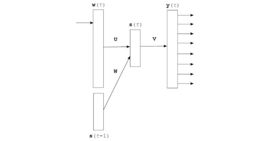 is the output from the previous time step and is the input of the current word vector (also converted via one-hot).
Input Layer: Similar to NNLM, the current time step needs to be converted to a word vector.
Hidden Layer: Perform a fully connected layer operation on the input and the hidden output from the previous time step.
-
Corresponding Dimensions:
Output Layer: A fully connected layer followed by a function to generate a probability distribution.
-
Where is a vector:
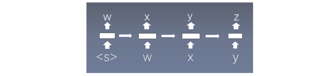
Each time step predicts a word; when predicting the nth word, it uses information from the previous n-1 words, without employing the Markov assumption, based on statistical principles. <S> indicates the start, the first word.
5.3 Word2vec Model
Log Linear Models definition: Establishing the language model as a multi-class problem, equivalent to a linear classifier plus softmax. Since only the softmax exponentiated part is nonlinear, adding the log makes it linear, hence the name log-linear model. The logistic regression model is a Log Linear Model.
The skip-gram and CBOW discussed in this section are also Log Linear Models.
5.3.1 Principles of Word2vec
Skip-gram Model:
-
Basic Idea of Language Model: The occurrence of the next word in a sentence is related to the preceding words, so the previous words can be used to predict the next word. The Markov assumption, such as in NNLM, and statistical thinking, predicts the next word based on all previous words, as in RNNLM. -
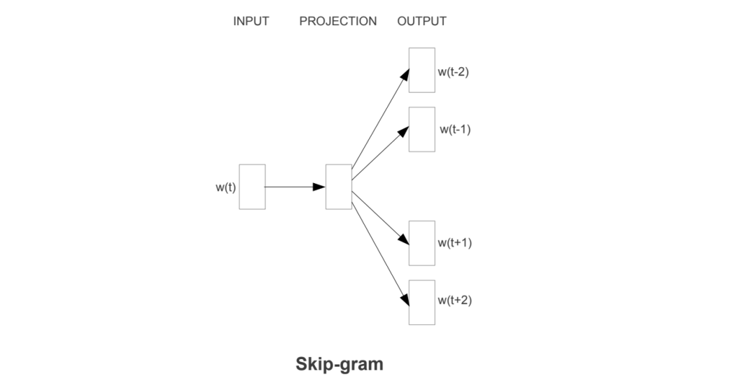
Basic Idea of Word2vec: Words that are close in a sentence are related; for example, after ‘today’, ‘morning’, ‘afternoon’, and ‘evening’ often appear. Therefore, the basic idea of Word2vec is to predict words using words; the skip-gram uses the center word to predict surrounding words, while CBOW uses surrounding words to predict the center word. The basic idea of Word2vec simplifies the language model.
5.3.2 Skip-gram
Calculation Process:
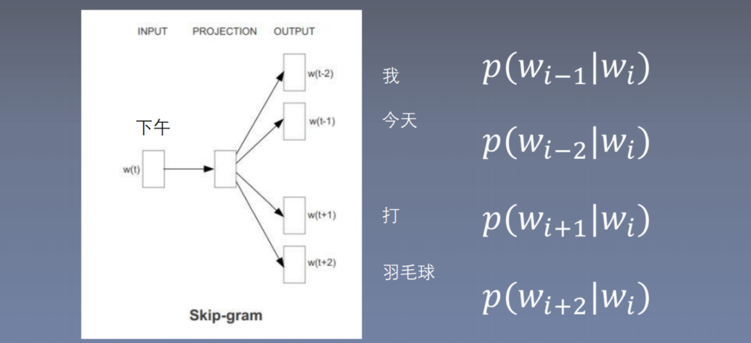
Skip-gram uses the center word to predict surrounding words. What is the range of center and surrounding words? Here, ‘afternoon’ is chosen as the center word with a window size of 2, thus predicting ‘I’, ‘today’, ‘hit’, and ‘play badminton’. Based on the window training size, four training samples are generated.
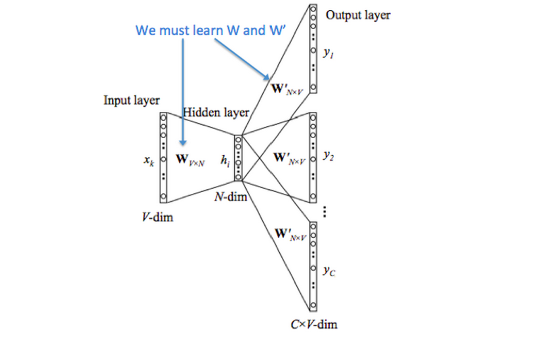
How to calculate the probabilities in the above diagram? In fact, probability issues in language models are a multi-class problem, where the input is the center word, and the label corresponds to a multi-class problem of vocabulary size. How to calculate probabilities and learn word vectors?
: Use the center word to predict surrounding words.
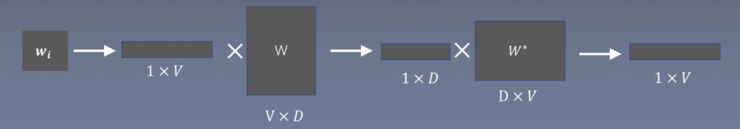
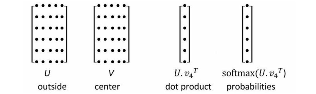
The input is an index representing the position of the word in the vocabulary, mapped to a 1×V one-hot vector; is the center word’s word vector matrix, dimension V×D, where each row represents a word vector; multiplying the one-hot vector with the center word’s word vector matrix yields a word vector; the resulting 1×D word vector is multiplied by the surrounding word’s word vector matrix to produce a 1×V vector. This vector, after softmax, gives the probability of each word, making the probability at the correct word’s position as large as possible.
The numerator: the surrounding word vector’s transpose multiplied by the center word vector.
Loss Function:
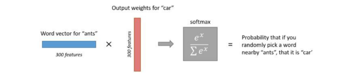
Simple and Intuitive but Inaccurate Explanation: In the vocabulary, take the center word ‘ants’ and all surrounding words, put them in a bag, and randomly select one; this word’s probability is that of ‘car’. This is similar to the occurrence matrix frequency. If ‘car’ and ‘ant’ both relate to the same word, they may have a certain dependency, thus potentially increasing accuracy, so this explanation is not precise.
To find the minimum:
-
is the center word vector -
is the surrounding word’s word vector in the context -
is the word vector of all surrounding words in the context -
is the window size
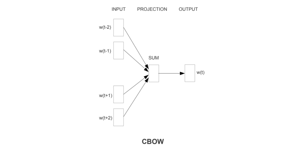
5.3.3 CBOW
Full name: Continuous Bag-of-Words Model, which ignores word order.
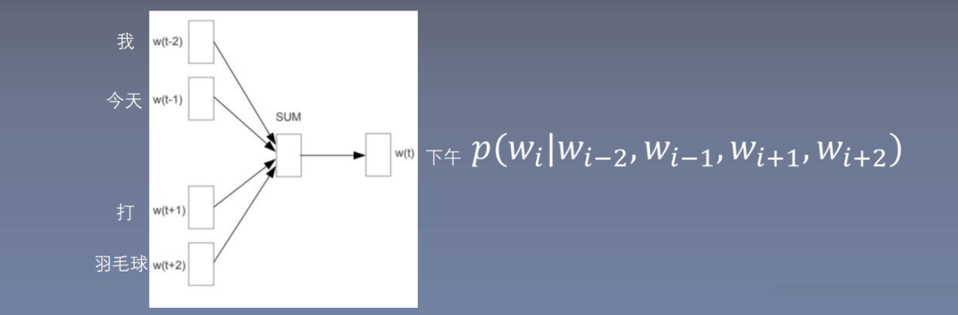
CBOW uses surrounding words to predict the center word. In NNLM, all inputs are concatenated together, resulting in a larger input, while averaging or summing the inputs results in a vector dimension the same as a single word vector, thus reducing model complexity. Here, summation is used.
For the center word, there is only one training sample.
:
The input index is converted to a 1×V one-hot vector.
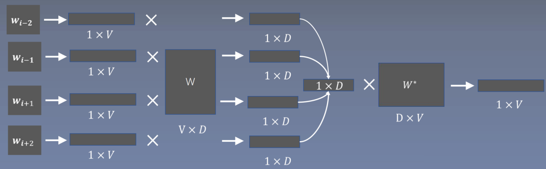
The input index represents the position of the word in the vocabulary, mapped to a 1×V one-hot vector; unlike Skip-gram, here is the surrounding word’s word vector matrix, dimension V×D, where each row represents a surrounding word’s word vector; multiplying the two yields each surrounding word’s word vector; after averaging or summing, the resulting 1×D vector is multiplied by the center word’s word vector matrix to produce a 1×V vector. This vector, after softmax, gives the probability of each word, maximizing the probability at the correct word’s position.
-
Context Words
-
is the sum of the surrounding context word vectors -
is the center word vector
6. Key Technologies
6.1 Complexity Discussion
How to reduce complexity?
Softmax outputs V probabilities:
is the surrounding word matrix, is the center word matrix, and the third matrix multiplication acts as a fully connected layer without activation functions or biases; the number of neurons in the fully connected layer equals the vocabulary size, as the softmax layer outputs many probabilities, which is very large, thus this fully connected layer is also very large. So how can we reduce complexity? Can we lower the complexity of softmax? The paper mentions two methods: hierarchical softmax and negative sampling.
6.2 Hierarchical Softmax
Transform softmax into multiple sigmoids, which can be represented in a binary tree format. Softmax requires multiple exponential operations, while sigmoid only requires one. As long as we convert to fewer exponential operations than softmax, we effectively accelerate computations.
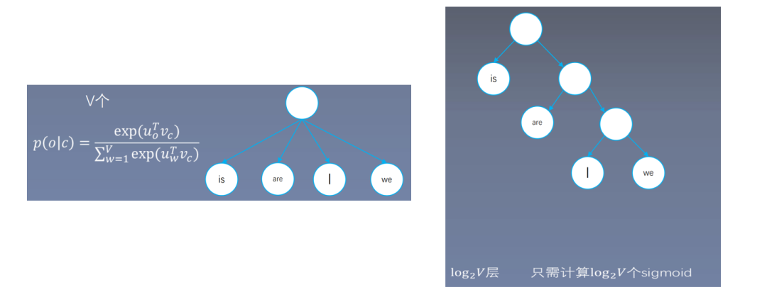
For layers, only calculations are needed.
6.2.1 Skip-gram Objective Function
Full Binary Tree: Why does hierarchical softmax require only calculations of sigmoids?
Only three steps are needed to find.
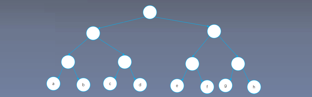
Assuming the vocabulary size is 8, softmax requires 8 exponential operations; if calculating sigmoid through an 8-node full binary tree, determining ‘a’ requires 3 binary classifications; determining ‘b’ also requires 3 binary classifications; thus, the classification count equals the depth of the tree minus 1.
Constructing Huffman Tree: A binary tree with the shortest weighted paths.
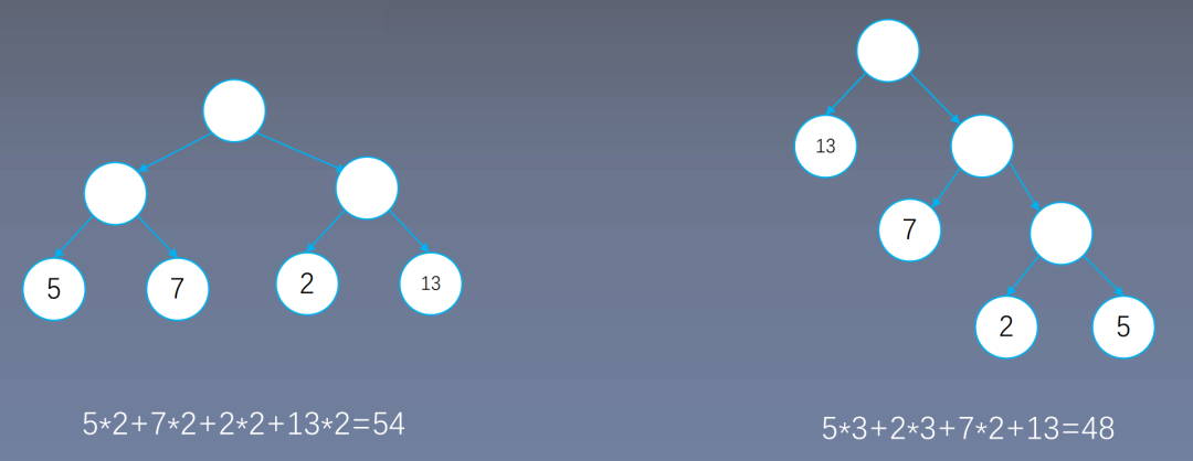
5 indicates that predicting this word requires 5 sigmoids; 7 means predicting this word requires 7 sigmoids; the number of edges represents the weight; the Huffman tree places high-frequency words at the top of the tree, reducing the number of operations.
Building the hierarchical softmax:
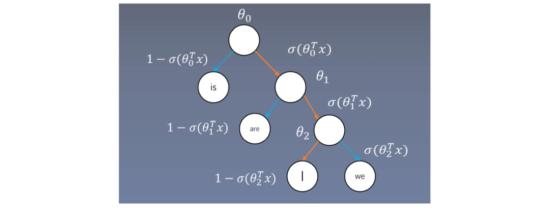
Each branch node is a vector; for example, in skip-gram, the center word vector is multiplied by the branch node, followed by sigmoid. If the result is less than zero, search left; if greater than zero, search right, and repeat with the next branch.
6.2.2 CBOW Hierarchical Softmax
Hierarchical softmax classification
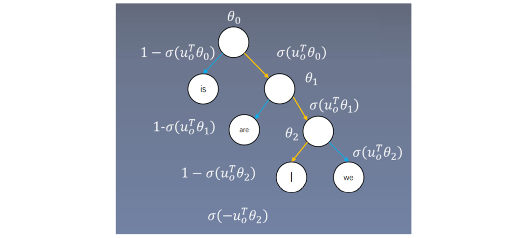
-
is the average of the surrounding context word vectors
Previously, both skip-gram and CBOW could yield final word vectors as the sum or average of the center and surrounding word vectors, but in hierarchical softmax, only one set of word vectors is present, as the count is less than that of the previous context, making the specific meaning unclear, possibly representing a cluster of word categories.
6.3 Negative Sampling (More Frequently Used)
In terms of both effectiveness and efficiency, negative sampling outperforms hierarchical softmax.
Abandon multi-class classification to enhance speed, transform multi-class into binary classification. A center word with surrounding words together forms a positive sample; for example, in the image, ‘jump over’ is a positive sample, while ‘jumps again’ is a negative sample, which may randomly select a center word with its surrounding words, but the vocabulary is very large, making this possibility negligible.

Basic idea: Increase the probability of positive samples and decrease the probability of negative samples.
For each word, one positive sample’s probability is output, but it is essential not to choose only one negative sample to avoid bias, as the positive sample is real while the negative sample is drawn from sampling. Generally, between 3-10 negative samples are chosen. If K negative samples are selected, the output consists of K probabilities, totaling probabilities, where K << V, and the result is better than multi-class classification. Here, the context word vector is still needed, with the matrix dimension being total parameters more than HS (hierarchical softmax) (each calculation is not much, whereas hierarchical softmax requires V probabilities, here only requires K).< /v$.
Loss function:
-
is the center word vector -
is the surrounding context word vector -
is the negative sampling context word vector
6.3.1 How to Sample?
The following diagram shows the curve:
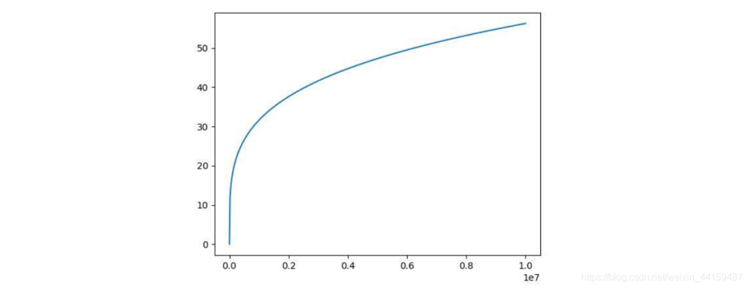
is the frequency of word in the dataset, is the normalized parameter, ensuring that the probability sum remains 1 after solving. The sampling probability of high-frequency words is reduced, while that of low-frequency words is increased. Since some unimportant words appear frequently (e.g., ‘the’, ‘a’), important words appear less frequently, which can accelerate training and yield better results.
6.3.2 CBOW Negative Sampling
Similarly, binary classification requires both positive and negative samples; the average of all surrounding word vectors combined with the true center word forms a positive sample, while the average of surrounding word vectors combined with randomly sampled words forms a negative sample.

The loss function is the same as above:
-
is the average of the surrounding context word vectors -
is the correct center word vector -
is the incorrect center word vector
6.4 High-Frequency Word Resampling (Subsampling of Frequent Words)
Consensus in Natural Language Processing: Words that appear with high frequency in documents or datasets often carry less information, such as ‘the’, ‘is’, ‘a’, ‘and’, while low-frequency words tend to carry more information.
What is a frog?
-
What is deep learning, what is CNN, what is RNN, this article tells you. -
Frog belongs to the phylum Chordata, class Amphibia, order Anura, family Ranidae, amphibians with no tail in adulthood, and lays eggs in water.
Reasons for resampling:
-
It is more beneficial to train important word pairs; for example, training the relationship between “France” and “Paris” is more useful than training between “France” and “the”. -
High-frequency words are quickly trained, while low-frequency words require more iterations.
Resampling method:
Where is the frequency of word in the dataset. In the text, is selected as , and the words in the training set will be deleted with a probability of .
Analysis of resampling: The higher the word frequency, the greater the probability of deletion. Conversely, if the word’s frequency is less than or equal to , then it will not be deleted.
Advantages: Accelerates training and results in better word vectors.
7. Model Complexity
7.1 Concept of Model Complexity
The complexity of the model also refers to temporal complexity:
-
is training complexity -
is the number of training epochs -
is the size of the dataset -
is model computational complexity, the time required for each training
Generally, the values of and in different algorithms are the same, often compared for size.
The method for calculating in the paper is unique, using the number of parameters to compute time complexity.
7.2 Time Complexity of Feedforward Network-Based Language Models
NNLM predicts the nth word based on the previous words:
| Layer Dimensions | Symbol Explanation |
|---|---|
| Dimensions Dimensions Dimensions | Number of preceding words Word vector dimensions Vocabulary size Hidden layer size |
Model complexity:
-
Input layer parameters: Input of words’ word vectors, each word mapped to a vector, for words it is -
Hidden layer parameters: The hidden layer input is , and the output neurons are , making the fully connected layer W dimensions -
is dimension -
If hierarchical softmax is used, each probability calculation requires an average of log2 V sigmoids, equivalent to log2 V multiplications with hidden outputs, where each count is equal to the number of hidden outputs, thus V×H becomes H×log2 V.
Bengio A neural probabilistic language model (2003)
7.3 Time Complexity of Recurrent Neural Network-Based Language Models
| Layer Dimensions | Symbol Explanation |
|---|---|
| Dimensions Dimensions Dimensions Dimensions Dimensions | Represents the current input word vector at time |
| Represents the previous output of the hidden layer | |
| Represents the index of the output word |
RNNLM model complexity:
7.4 Skip-gram Complexity
7.4.1 Hierarchical Softmax Complexity
For the original skip-gram, its center word vector is dimension, then multiplied by (dimension, generating probabilities), and for a center word, it corresponds to multiple surrounding words, generally 5-10, assuming here, thus multiplying yields the first formula in the above image. If hierarchical softmax is used, it becomes.
7.4.2 Negative Sampling Complexity
For each center word, there is one positive sample and K negative samples, each becoming a D-dimensional word vector, resulting in the second formula in the above image.
7.5 CBOW Complexity
CBOW complexity:
In the original CBOW, the input is the surrounding words, with each surrounding word having dimension, thus the surrounding words yield dimension, followed by a feedforward layer producing a vector of vocabulary size, hence the intermediate matrix dimension is, resulting in total parameters.
Similar to skip-gram, CBOW corresponds to the complexity of hierarchical softmax and negative sampling:
Hierarchical softmax:
Negative sampling:
Note: The above represents the parameters needed for each calculation.
7.6 Model Complexity Comparison
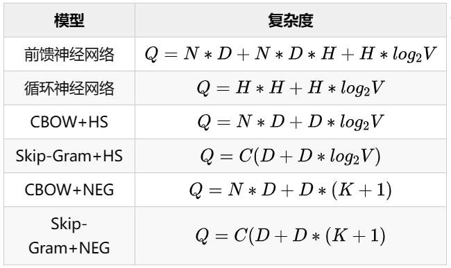
Theoretical analysis shows that both hierarchical softmax and negative sampling are faster than feedforward and recurrent neural networks, with CBOW being faster than Skip-Gram; negative sampling is faster than hierarchical softmax.
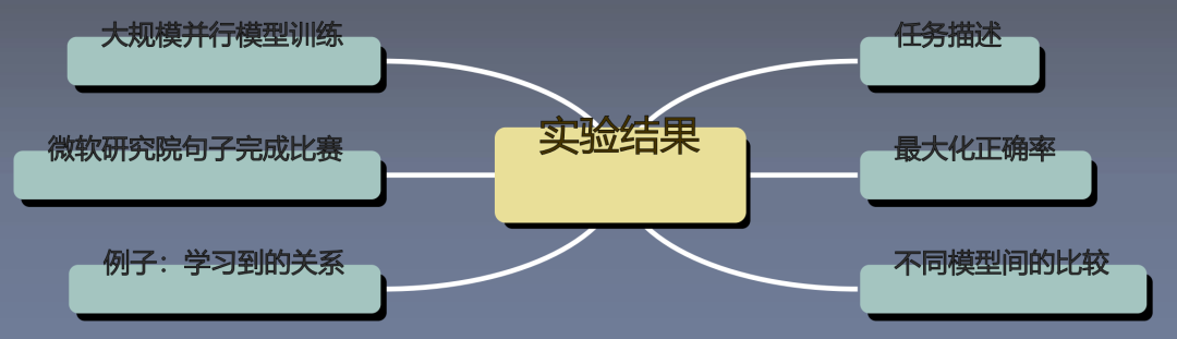
8. Experimental Result Analysis
8.1 Task Description
The task is a word pair inference task; the first five in the diagram are semantic classes, and the last nine are grammatical classes.
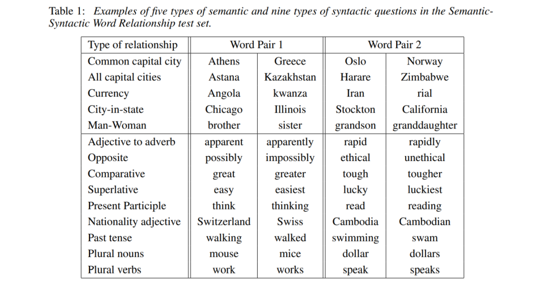
Grammatical class data is easy to collect, while semantic class data is challenging to gather.
| Relation Type | Translation |
|---|---|
| capital-common-countries | Common Country Capitals |
| capital-world | Capitals of Various Countries |
| currency | Currency |
| city-in-state | State-City |
| family | Family Relations |
| gram1-adjective-to-adverb | Adjective-Adverb |
| gram2-opposite | Antonyms |
| gram3-comparative | Comparative |
| gram4-superlative | Superlative |
| gram5-present-participle | Present Participle |
| gram6-nationality-adjective | Nationality Adjective |
| gram7-past-tense | Past Tense |
| gram8-plural | Plural |
| gram9-plural-verb | Third Person Singular |
Word2vec program questions-words.txt:
// Copyright 2013 Google Inc. All Rights Reserved.
: capital-common-countries
Athens Greece Baghdad Iraq
Athens Greece Bangkok Thailand
Athens Greece Beijing China
Athens Greece Berlin Germany
Athens Greece Bern Switzerland
Athens Greece Cairo Egypt
Athens Greece Canberra Australia
Athens Greece Hanoi Vietnam
Athens Greece Havana Cuba
Athens Greece Helsinki Finland
...
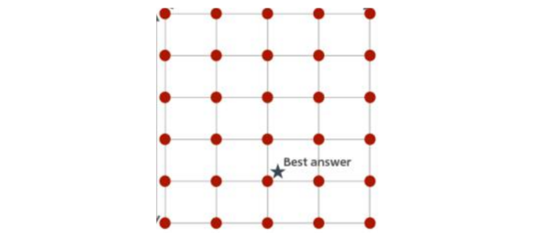
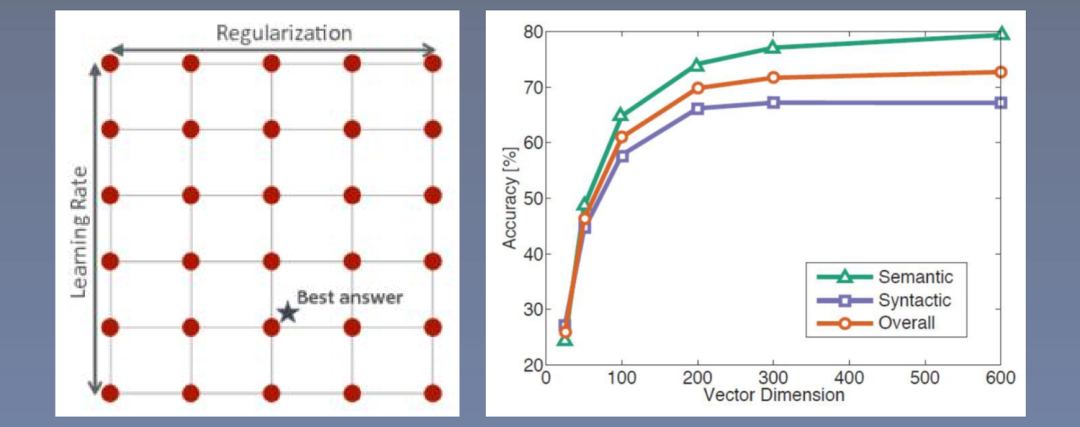
8.2 Maximizing Accuracy (Parameter Optimization)
Using a small dataset to tune parameters, selecting the best parameters, which include dimension and training data size, are the two parameters to find.
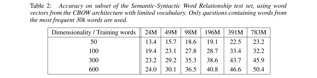
As the dimension increases (vertical axis) and the dataset expands (horizontal axis), the performance generally improves.
8.3 Model Comparison
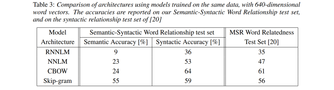
The MSR Word Relatedness test set mainly consists of grammatical data. Both RNNLM and NNLM perform well in semantic accuracy, while CBOW also does well, and skip-gram performs well in both grammatical and semantic accuracy.
RNNLM took 8 weeks on a single machine, while NNLM had a larger computation load.
RNN performs relatively better on grammatical issues, NNLM performs better overall, and CBOW performs well.
Skip-gram is more balanced, performing well in semantic issues.
LDC corpora 320M words, 82K
Comparing with open-source word vectors from others:
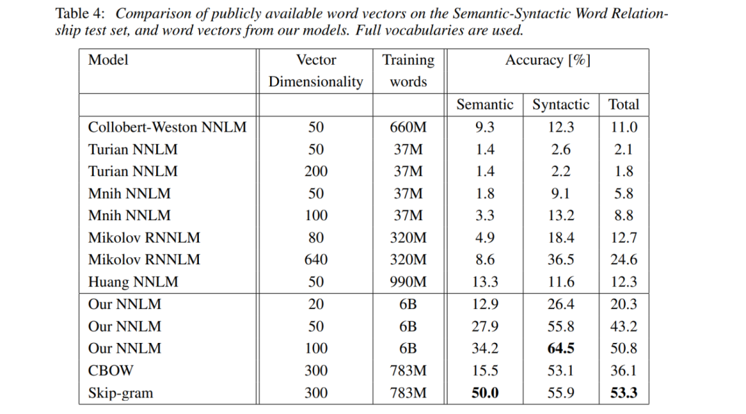
Our NNLM utilized hierarchical softmax for acceleration.
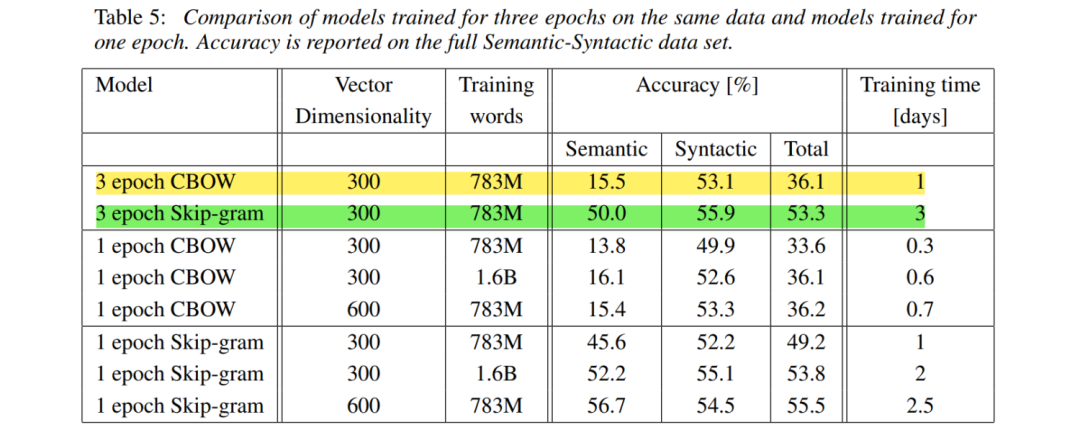
3 epochs of CBOW (36.1) < 1 epoch of skip-gram (49.2)
3 epochs of 300dim < 1 epoch of 600d
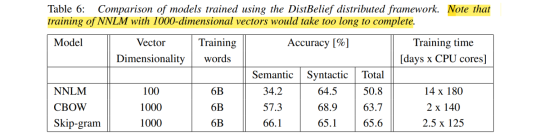
8.4 Large Scale Parallel Model Training
Large Scale Parallel Training of Model
8.5 Microsoft Research Sentence Completion Competition
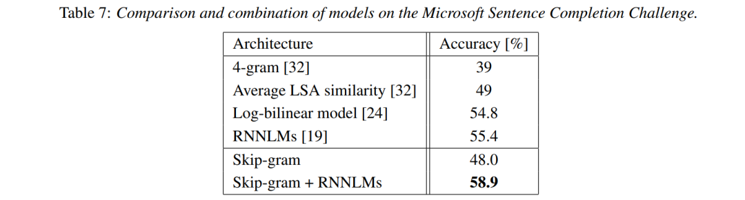
Similar to a fill-in-the-blank task, one word in a sentence is covered, and five prediction results are provided.
Skip-gram only counts surrounding words without utilizing the relationships between words, so it can be trained jointly with the RNNLM language model.
8.6 HS and NEG Comparison
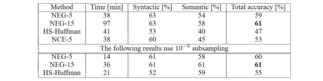
NCE: Other negative sampling methods.
The table below shows the use of resampling, significantly improving speed.
Example: Learned relationships
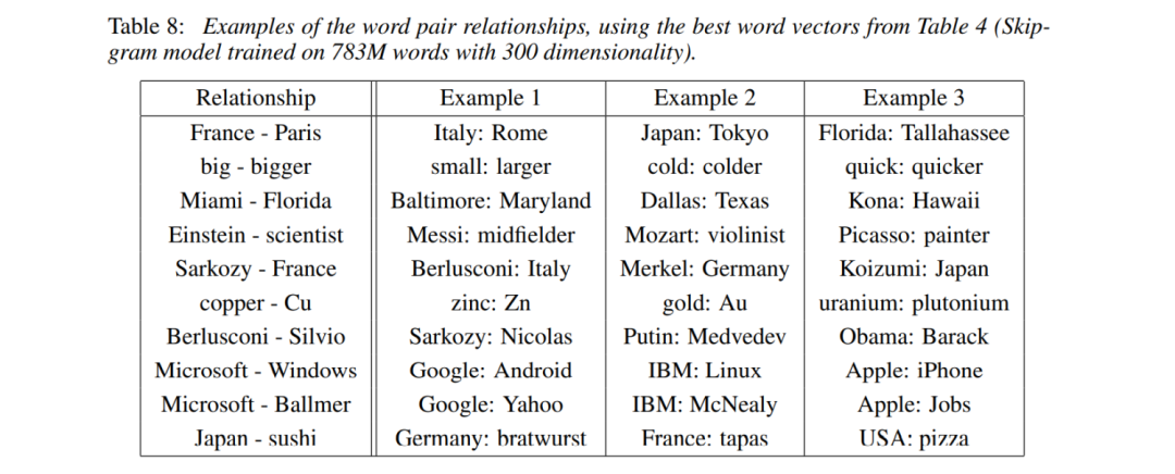
Averaging the learned relationships of ten word pairs can offset deviations.
Out-of-the-list words: Words that do not fit the current category.
9. Discussion and Conclusion
Discussing the issues within the paper and summarizing what has been learned in this phase.
9.1 Discussion
Hyperparameter Selection: When using gensim to perform word2vec, is there a good correlation range between the dimension of word vectors and the number of words?
Dimension is generally chosen between 100-500, with an initial value set to the 1/4th power of vocabulary size V, e.g., V=10K, dim=100. min_count is generally chosen between 2-10, representing the minimum frequency of words in the corpus, discarding words below this frequency, determining vocabulary size.
gridsearch
9.2 Conclusion
Main Innovations of the Paper: 1. Proposes a new structure: This structure uses words to predict words rather than using a series of preceding words to predict a word, simplifying the structure. It also introduces hierarchical softmax and negative sampling, significantly reducing computational load, allowing for higher dimensions and larger datasets.
2. Utilizes distributed training frameworks: Training on large data for better results.
3. Introduces new word similarity tasks: Analogy word categories.
Key Points:
-
A simpler prediction model — word2vec -
A faster classification scheme — HS and NEG
Innovations:
-
Replacing language model predictions with word pair predictions -
Using HS and NEG to reduce classification complexity -
Utilizing subsampling to accelerate training -
A new word pair inference dataset to objectively evaluate word vector quality
Insights:
1. Simple models on large datasets often outperform complex models on small datasets.
simple models trained on huge amounts of data outperform complex systems trained on less data. (1 Introduction p1)
2. The vector of “King” minus the vector of “Man” plus the vector of “Woman” is closest to the vector representation of the word “Queen”.
vector(“King”) – vector(“Man”) + vector(“Woman”) results in a vector that is closest to the vector representation of the word “Queen” (1.1 Goals of the Paper p3)
It indicates that word2vec can effectively learn algebraic relationships between word pairs, and since neural networks involve calculations between numbers, if they can learn algebraic relationships between word vectors, they are very useful for neural networks.
3. We decided to design simple models to train word vectors; although simple models may not represent data as accurately as neural networks, they can train on much more data quickly.
we decided to explore simpler models that might not be able to represent the data as precisely as neural networks, but can possibly be trained on much more data efficiently (3 New Log-linear Models p1)
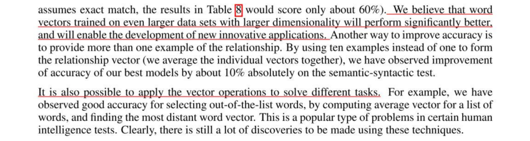
4. We believe that using larger word vector dimensions on larger datasets will yield better word vectors.
We believe that word vectors trained on even larger data sets with larger dimensionality will perform significantly better (5 Examples of the Learned Relationships p1)
Click here 👇 to follow me for weekly updates on AI technology insights!
Previous Exciting Readings
👉 Kaggle competition baseline collection
👉 Classic paper recommendations collection
👉 Essential AI reading books
👉 Learning experiences for undergraduate and graduate students