Understanding Vision Transformers in Deep Learning

Since the concept of “Attention is All You Need” was introduced in 2017, the Transformer model has quickly emerged in the field of Natural Language Processing (NLP), establishing its leading position. By 2021, the idea that “one image is equivalent to 16×16 words” successfully brought the Transformer model into computer vision tasks. Since then, numerous Transformer-based architectures have emerged and been applied in the field of computer vision.

This article will detail the Vision Transformer (ViT) described in “one image is equivalent to 16×16 words”, including its open-source code and conceptual explanations of various components. All code is implemented using the PyTorch Python package.

This article is one of a series of in-depth studies on the internal workings of Vision Transformers, providing an executable code version in Jupyter Notebook. Other articles in the series include: Analysis of Vision Transformers, Application of Attention Mechanism in Vision Transformers, Analysis of Position Encoding in Vision Transformers, Tokens-to-Token Vision Transformers Analysis, and the GitHub repository for the Vision Transformers analysis series.

So, what are Vision Transformers? As introduced in “Attention is All You Need”, Transformers are machine learning models that utilize attention mechanisms as their primary learning mechanism. They quickly became the leading technology for sequence-to-sequence tasks (such as language translation).

The concept of “one image is equivalent to 16×16 words” successfully improved the Transformer proposed in [1] to handle image classification tasks, giving rise to the Vision Transformer (ViT). Like the Transformer in [1], ViT is based on the attention mechanism. However, unlike the Transformer used for NLP tasks, which contains both encoder and decoder attention branches, ViT only uses the encoder. The output of the encoder is then passed to a neural network “head” for prediction.

However, the ViT implemented in “one image is equivalent to 16×16 words” has a drawback: its optimal performance requires pre-training on large datasets. The best model was pre-trained on the proprietary JFT-300M dataset. In contrast, models pre-trained on the smaller open-source ImageNet-21k dataset perform comparably to the state-of-the-art convolutional ResNet models.

Tokens-to-Token ViT: Training Vision Transformers from Scratch on ImageNet attempts to eliminate this pre-training requirement by introducing a novel preprocessing method that converts input images into a series of tokens. For more information on this method, please refer to the relevant literature. In this article, we will focus on the ViT implemented in “one image is equivalent to 16×16 words”.

Model Analysis

This article follows the model structure outlined in “one image is equivalent to 16×16 words”. However, the code from that paper has not been publicly released. The recent code from “Tokens-to-Token ViT” can be found on GitHub. The Tokens-to-Token ViT (T2T-ViT) model adds a Tokens-to-Token (T2T) module before the standard ViT backbone structure. The code in this article is based on the ViT components from the “Tokens-to-Token ViT” GitHub code. Modifications have been made to the code to allow for non-square input images and to remove dropout layers.

The structure diagram of the ViT model is shown below.

Understanding Vision Transformers in Deep Learning

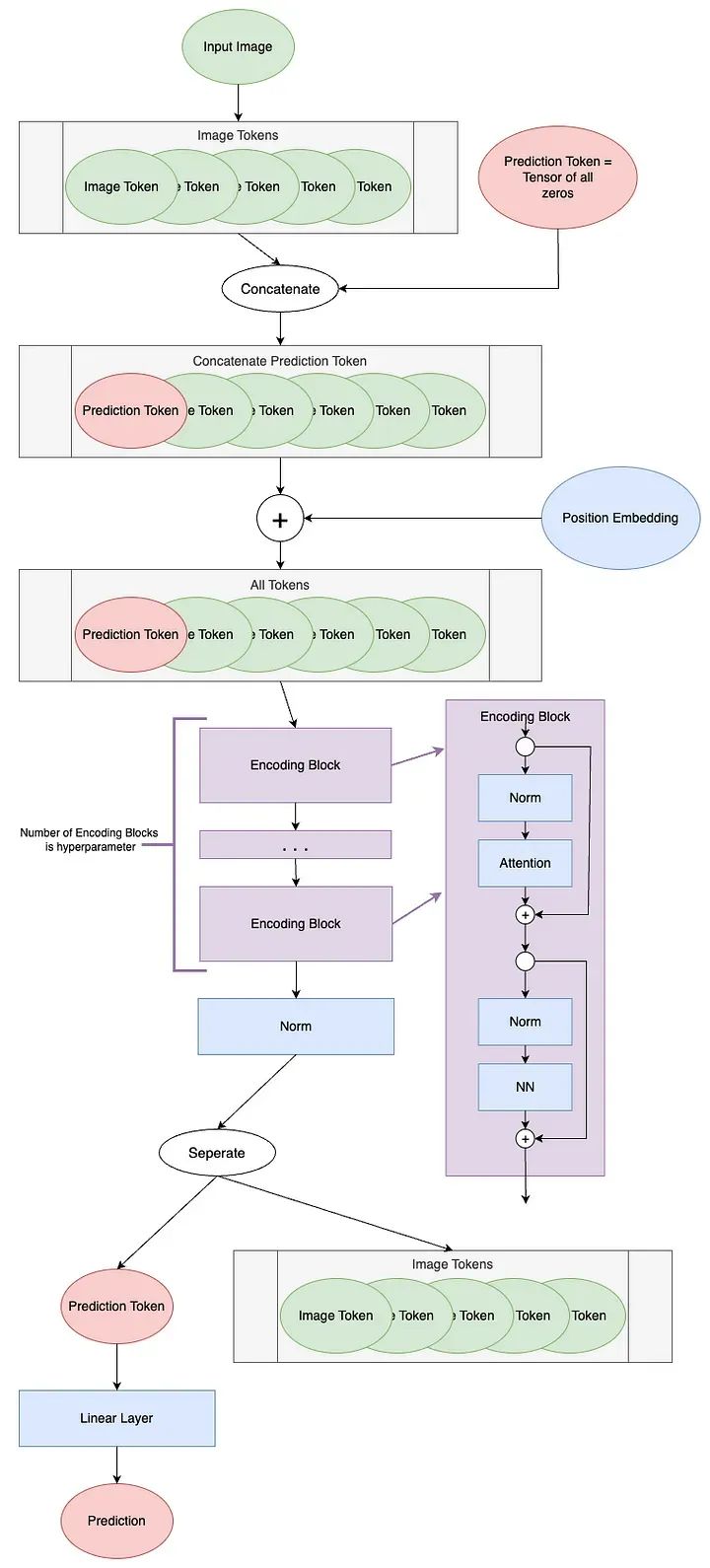
ViT model diagram

Image Tokenization

The first step of ViT is to create tokens from the input image. Transformers operate on a series of tokens; in NLP, this is typically the words of a sentence. For computer vision, how to segment the input into tokens is not very clear. ViT converts images into tokens such that each token represents a local area (or patch) of the image. They describe how to reshape an image with height H, width W, and C channels into N patches of size P:

Each token has a length of P²*C. Let’s take this pixel art “Mountain at Dusk” (by Luis Zuno) as an example for patch tokenization. The original artwork has been cropped and converted to a single-channel image. This means that the value of each pixel is between 0 and 1. Single-channel images are usually displayed in grayscale, but we will show it in a purple color scheme for better visibility. Note that the patch tokenization is not included in the code related to [3].

mountains = np.load(os.path.join(figure_path, 'mountains.npy'))H = mountains.shape[0]W = mountains.shape[1]print('Mountain at Dusk is H =', H, 'and W =', W, 'pixels.')

<span>print('

')</span>

fig = plt.figure(figsize=(10,6))plt.imshow(mountains, cmap='Purples_r')plt.xticks(np.arange(-0.5, W+1, 10), labels=np.arange(0, W+1, 10))plt.yticks(np.arange(-0.5, H+1, 10), labels=np.arange(0, H+1, 10))plt.clim([0,1])cbar_ax = fig.add_axes([0.95, .11, 0.05, 0.77])plt.clim([0, 1])plt.colorbar(cax=cbar_ax);#plt.savefig(os.path.join(figure_path, 'mountains.png'))

Mountain at Dusk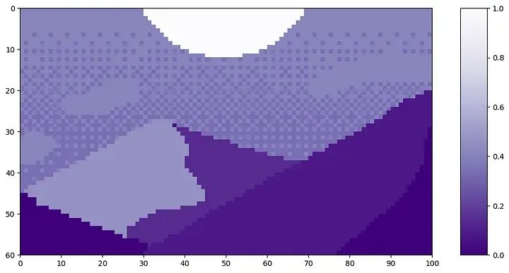 is H = 60 and W = 100 pixels.

The height of this image is H=60, and the width is W=100. We will set P=20, as it can evenly divide H and W.

P = 20N = int((H*W)/(P**2))print('There will be', N, 'patches, each', P, 'by', str(P)+'.')

<span>print('

')</span>

fig = plt.figure(figsize=(10,6))plt.imshow(mountains, cmap='Purples_r')plt.hlines(np.arange(P, H, P)-0.5, -0.5, W-0.5, color='w')plt.vlines(np.arange(P, W, P)-0.5, -0.5, H-0.5, color='w')plt.xticks(np.arange(-0.5, W+1, 10), labels=np.arange(0, W+1, 10))plt.yticks(np.arange(-0.5, H+1, 10), labels=np.arange(0, H+1, 10))x_text = np.tile(np.arange(9.5, W, P), 3)y_text = np.repeat(np.arange(9.5, H, P), 5)for i in range(1, N+1): plt.text(x_text[i-1], y_text[i-1], str(i), color='w', fontsize='xx-large', ha='center')plt.text(x_text[2], y_text[2], str(3), color='k', fontsize='xx-large', ha='center');#plt.savefig(os.path.join(figure_path, 'mountain_patches.png'), bbox_inches='tight'

There will be 15 patches, each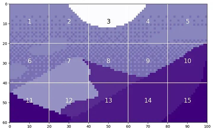 20 by 20.

By flattening these patches, we can see the generated Token. Let’s take the 12th patch as an example, as it contains four different tones.

<span><span>print</span>(<span>'Each patch will make a token of length'</span>, str(P**<span>2</span>)+<span>'.'</span>)</span>

<span><span>print</span>(<span>'

'</span>)</span>

patch12 = mountains[40:60, 20:40]token12 = patch12.reshape(1, P**2)fig = plt.figure(figsize=(10,1))plt.imshow(token12, aspect=10, cmap='Purples_r')plt.clim([0,1])

<span>plt.xticks(np.arange(<span>-0.5</span>, <span>401</span>, <span>50</span>), labels=np.arange(<span>0</span>, <span>401</span>, <span>50</span>))</span>

plt.yticks([]);

<span>#plt.savefig(os.path.join(figure_path, <span>'mountain_token12.png'</span>), bbox_inches=<span>'tight'</span>)</span>

Each patch will make a token of length 400.

Understanding Vision Transformers in Deep Learning

After extracting tokens from the image, a linear projection is typically used to change the length of the tokens. This is achieved through a learnable linear layer. The new token length is referred to as the latent dimension, channel dimension, or token length. After projection, the tokens can no longer be visually recognized as patches of the original image. Now that we understand this concept, we can look at how patch tokenization is implemented in code.

class Patch_Tokenization(nn.Module):

<span> <span><span>def</span> <span>__init__</span><span>(<span>self</span>,</span></span></span><code><span> <span>img_size:</span> tuple[int, int, int]=(<span>1</span>, <span>1</span>, <span>60</span>, <span>100</span>)</span>,

 patch_size: int=50, token_len: int=768): """ Patch Tokenization Module Args: img_size (tuple[int, int, int]): size of input (channels, height, width) patch_size (int): the side length of a square patch token_len (int): desired length of an output token """""" super().__init__() ## Defining Parameters self.img_size = img_size C, H, W = self.img_size self.patch_size = patch_size self.token_len = token_len

<span>        assert H % <span>self</span>.patch_size == <span>0</span>, <span>'Height of image must be evenly divisible by patch size.'</span></span>

<span>        assert W % <span>self</span>.patch_size == <span>0</span>, <span>'Width of image must be evenly divisible by patch size.'</span></span>

 self.num_tokens = (H / self.patch_size) * (W / self.patch_size) ## Defining Layers

<span> <span>self</span>.split = nn.Unfold(kernel_size=<span>self</span>.patch_size, stride=<span>self</span>.patch_size, padding=<span>0</span>)</span>

 self.project = nn.Linear((self.patch_size**2)*C, token_len) def forward(self, x): x = self.split(x).transpose(1,0) x = self.project(x) return x

Note the two assertion statements that ensure the image dimensions are divisible by the patch size. The actual patch division is implemented through a torch.nn.Unfold⁵ layer.

We will use the cropped single-channel version of Mountain at Dusk⁴ to run an example of this code. We should see the same number of Token and initial Token size values as before. We will use token_len=768 as the projection length, which is the size of the base variant of ViT².

The first line in the code block below changes the data type of Mountain at Dusk⁴ from a NumPy array to a Torch tensor. We also need to perform an unsqueeze⁶ operation on the tensor to create a channel dimension and a batch size dimension. As above, we only have one channel. Since there is only one image, the batch size is 1.

x = torch.from_numpy(mountains).unsqueeze(0).unsqueeze(0).to(torch.float32)token_len = 768

<span>print('Input dimensions are

	batchsize:', x.shape[0], '

	number of input channels:', x.shape[1], '

	image size:', (x.shape[2], x.shape[3]))</span>

# Define the Modulepatch_tokens = Patch_Tokenization(img_size=(x.shape[1], x.shape[2], x.shape[3]), patch_size = P, token_len = token_len)

Input dimensions are batchsize: 1 number of input channels: 1 image size: (60, 100)

Now, we will divide the image into Tokens.

x = patch_tokens.split(x).transpose(2,1)

<span>print('After patch tokenization, dimensions are

	batchsize:', x.shape[0], '

	number of tokens:', x.shape[1], '

	token length:', x.shape[2])</span>

After patch tokenization, dimensions are batchsize: 1 number of tokens: 15 token length: 400

As we saw in the example, there are a total of N=15 tokens of length 400. Finally, we will project the Tokens to token_len.

x = patch_tokens.split(x).transpose(2,1)

<span><span>print</span>(<span>'After patch tokenization, dimensions are

	batchsize:'</span>, x.shape[<span>0</span>], <span>'

	number of tokens:'</span>, x.shape[<span>1</span>, <span>'

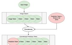
	token length:'</span>, x.shape[<span>2</span>])</span>

Now that we have the Tokens, we are ready to proceed with ViT.

Token Processing

We will refer to the next two steps of ViT, which occur before the encoding blocks, as “Token Processing”. The components of Token Processing in the ViT diagram are shown below.

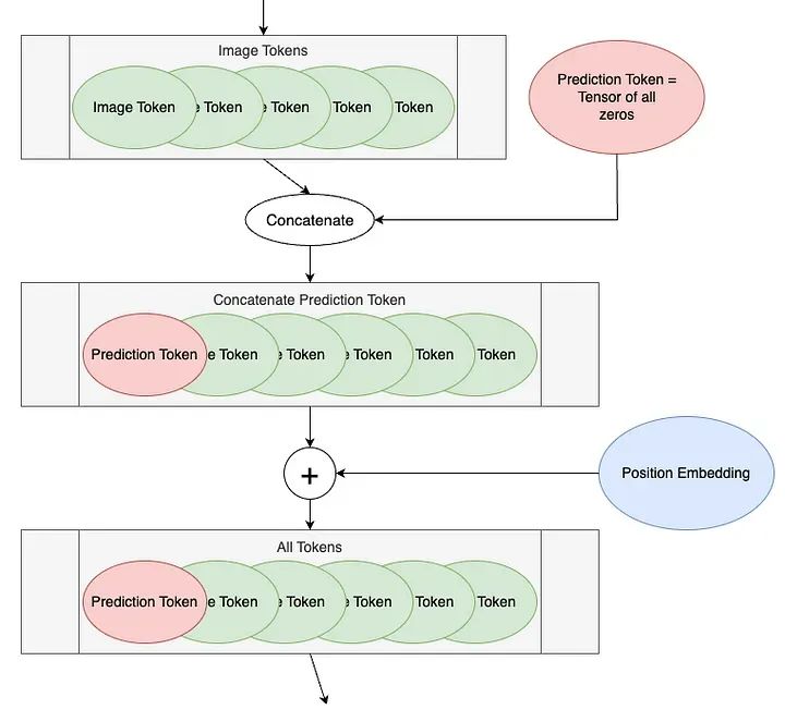Understanding Vision Transformers in Deep Learning The first step is to add a blank Token before the image Token, called the Prediction Token. This Token will be used to output the encoding blocks for prediction. It is initially blank—equivalent to zero—so it can gather information from other image Tokens.

# Define an Inputnum_tokens = 175token_len = 768batch = 13x = torch.rand(batch, num_tokens, token_len)

<span><span>print</span>(<span>'Input dimensions are

	batchsize:'</span>, x.shape[0], <span>'

	number of tokens:'</span>, x.shape[1], <span>'

	token length:'</span>, x.shape[2])</span>

# Append a Prediction Tokenpred_token = torch.zeros(1, 1, token_len).expand(batch, -1, -1)

<span><span>print</span>(<span>'Prediction Token dimensions are

	batchsize:'</span>, pred_token.shape[0], <span>'

	number of tokens:'</span>, pred_token.shape[1], <span>'

	token length:'</span>, pred_token.shape[2])</span>

x = torch.cat((pred_token, x), dim=1)

<span><span>print</span>(<span>'Dimensions with Prediction Token are

	batchsize:'</span>, x.shape[0], <span>'

	number of tokens:'</span>, x.shape[1], <span>'

	token length:'</span>, x.shape[2])</span>

Input dimensions are batchsize: 13 number of tokens: 175 token length: 768Prediction Token dimensions are batchsize: 13 number of tokens: 1 token length: 768Dimensions with Prediction Token are batchsize: 13 number of tokens: 176 token length: 768

We will start with 175 Tokens. Each Token has a length of 768, which is the size of the base variant of ViT². We use a batch size of 13 because it is prime and does not confuse with any other parameters.

def get_sinusoid_encoding(num_tokens, token_len): """ Make Sinusoid Encoding Table Args: num_tokens (int): number of tokens token_len (int): length of a token Returns: (torch.FloatTensor) sinusoidal position encoding table """ def get_position_angle_vec(i):

<span> <span>return</span> [i / np.power(<span>10000</span>, <span>2</span> * (j // <span>2</span>) / token_len) <span>for</span> j <span>in</span> range(token_len)]</span>

<span>    sinusoid_table = np.array([get_position_angle_vec(i) <span>for</span> i <span>in</span> range(num_tokens)])</span>

<span>    sinusoid_table[:, <span>0</span>::<span>2</span>] = np.sin(sinusoid_table[:, <span>0</span>::<span>2</span>])</span>

<span>    sinusoid_table[:, <span>1</span>::<span>2</span>] = np.cos(sinusoid_table[:, <span>1</span>::<span>2</span>]) </span>

 return torch.FloatTensor(sinusoid_table).unsqueeze(0)PE = get_sinusoid_encoding(num_tokens+1, token_len)

<span>print(<span>'Position embedding dimensions are

	number of tokens:'</span>, PE.shape[<span>1</span>, <span>'

	token length:'</span>, PE.shape[<span>2</span>])</span>

x = x + PE

<span>print(<span>'Dimensions with Position Embedding are

	batchsize:'</span>, x.shape[<span>0</span>, <span>'

	number of tokens:'</span>, x.shape[<span>1</span>, <span>'

	token length:'</span>, x.shape[<span>2</span>])</span>

Position embedding dimensions are number of tokens: 176 token length: 768Dimensions with Position Embedding are batchsize: 13 number of tokens: 176 token length: 768

Now we have added a position embedding to our Tokens. Position embeddings allow the Transformer to understand the order of the image tokens. Note that this is an addition, not a concatenation. The specifics of position embeddings are worth discussing later.

<span> <span>return</span> [i / np.power(<span>10000</span>, <span>2</span> * (j // <span>2</span>) / token_len) <span>for</span> j <span>in</span> range(token_len)]</span>

<span>    sinusoid_table = np.array([get_position_angle_vec(i) <span>for</span> i <span>in</span> range(num_tokens)])</span>

<span>    sinusoid_table[:, <span>0</span>::<span>2</span>] = np.sin(sinusoid_table[:, <span>0</span>::<span>2</span>])</span>

<span>    sinusoid_table[:, <span>1</span>::<span>2</span>] = np.cos(sinusoid_table[:, <span>1</span>::<span>2</span>]) </span>

 return torch.FloatTensor(sinusoid_table).unsqueeze(0)PE = get_sinusoid_encoding(num_tokens+1, token_len)

<span>print(<span>'Position embedding dimensions are

	number of tokens:'</span>, PE.shape[<span>1</span>, <span>'

	token length:'</span>, PE.shape[<span>2</span>])</span>

x = x + PE

<span>print(<span>'Dimensions with Position Embedding are

	batchsize:'</span>, x.shape[<span>0</span>, <span>'

	number of tokens:'</span>, x.shape[<span>1</span>, <span>'

	token length:'</span>, x.shape[<span>2</span>])</span>

Now, our Tokens are ready to enter the encoding blocks.

Encoding Blocks

The encoding blocks are where the model actually learns from the image tokens. The number of encoding blocks is a hyperparameter set by the user. The diagram of the encoding blocks is shown below.

Understanding Vision Transformers in Deep Learning

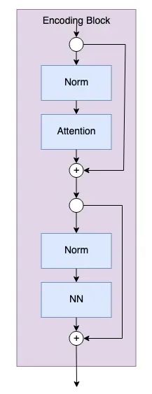
The code for the encoding blocks is as follows.

<span><span>class</span> <span>Encoding(nn.Module):    def __init__(self,       dim: int,       num_heads: int=1,       hidden_chan_mul: float=4.,       qkv_bias: bool=False,       qk_scale: NoneFloat=None,       act_layer=nn.GELU,        norm_layer=nn.LayerNorm):                """ Encoding Block            Args:                dim (int): size of a single token                num_heads(int): number of attention heads in MSA                hidden_chan_mul (float): multiplier to determine the number of hidden channels (features) in the NeuralNet component                qkv_bias (bool): determines if the qkv layer learns an addative bias                qk_scale (NoneFloat): value to scale the queries and keys by;                                     if None, queries and keys are scaled by ``head_dim ** -0.5``                act_layer(nn.modules.activation): torch neural network layer class to use as activation                norm_layer(nn.modules.normalization): torch neural network layer class to use as normalization        """        super().__init__()        ## Define Layers        self.norm1 = norm_layer(dim)        self.attn = Attention(dim=dim,                            chan=dim,                            num_heads=num_heads,                            qkv_bias=qkv_bias,                            qk_scale=qk_scale)        self.norm2 = norm_layer(dim)        self.neuralnet = NeuralNet(in_chan=dim,                                hidden_chan=int(dim*hidden_chan_mul),                                out_chan=dim,                                act_layer=act_layer)    def forward(self, x):        x = x + self.attn(self.norm1(x))        x = x + self.neuralnet(self.norm2(x))        return x</span></span>

num_heads 、qkv_bias和qk_scale参数定义了注意力模块组件。关于视觉转换器的注意力的深入研究留待下次再讨论。

hidden_ chan_mul和act_layer参数定义神经网络模块组件。激活层可以是任意⁷层。我们稍后torch.nn.modules.activation会详细介绍神经网络模块。

可以从任意⁸层中选择norm_layer torch.nn.modules.normalization。

现在，我们将逐步介绍图中的每个蓝色块及其附带的代码。我们将使用长度为 768 的 176 个标记。我们将使用批处理大小 13，因为它是素数，不会与任何其他参数混淆。我们将使用 4 个注意力头，因为它可以均匀划分标记长度；但是，您不会在编码块中看到注意力头维度。

<span><span># Define an Inputnum_tokens = 176token_len = 768batch = 13heads = 4x = torch.rand(batch, num_tokens, token_len)print('Input dimensions are

	batchsize:', x.shape[0], '

	number of tokens:', x.shape[1], '

	token length:', x.shape[2])# Define the ModuleE = Encoding(dim=token_len, num_heads=heads, hidden_chan_mul=1.5, qkv_bias=False, qk_scale=None, act_layer=nn.GELU, norm_layer=nn.LayerNorm)E.eval();</span></span>

<span><span>Input</span> <span>dimensions are   batchsize: 13    number of tokens: 176    token length: 768</span></span>

现在，我们将通过一个规范层和一个注意力模块。编码块中的注意力模块是参数化的，因此它不会改变标记长度。在注意力模块之后，我们实现了第一个拆分连接。

<span>y = E.norm1(x)<span>print</span>(<span>'After norm, dimensions are

	batchsize:'</span>, y.shape[0], <span>'

	number of tokens:'</span>, y.shape[1], <span>'

	token size:'</span>, y.shape[2])y = E.attn(y)<span>print</span>(<span>'After attention, dimensions are

	batchsize:'</span>, y.shape[0], <span>'

	number of tokens:'</span>, y.shape[1], <span>'

	token size:'</span>, y.shape[2])y = y + xprint(<span>'After split connection, dimensions are

	batchsize:'</span>, y.shape[0], <span>'

	number of tokens:'</span>, y.shape[1], <span>'

	token size:'</span>, y.shape[2])</span>

<span><span>After</span> <span>norm, dimensions are   batchsize: 13    number of tokens: 176    token size: 768After attention, dimensions are   batchsize: 13    number of tokens: 176    token size: 768After split connection, dimensions are   batchsize: 13    number of tokens: 176    token size: 768</span></span>

现在，我们经过另一个规范层，然后是神经网络模块。最后是第二个拆分连接。

z = E.norm2(y)

<span><span>print</span>(<span>'After norm, dimensions are

	batchsize:'</span>, z.shape[0], <span>'

	number of tokens:'</span>, z.shape[1], <span>'

	token size:'</span>, z.shape[2])</span>

z = E.neuralnet(z)

<span><span>print</span>(<span>'After neural net, dimensions are

	batchsize:'</span>, z.shape[0], <span>'

	number of tokens:'</span>, z.shape[1], <span>'

	token size:'</span>, z.shape[2])</span>

z = z + y

<span><span>print</span>(<span>'After split connection, dimensions are

	batchsize:'</span>, z.shape[0], <span>'

	number of tokens:'</span>, z.shape[1], <span>'

	token size:'</span>, z.shape[2])</span>

After norm, dimensions are batchsize: 13 number of tokens: 176 token size: 768After neural net, dimensions are batchsize: 13 number of tokens: 176 token size: 768After split connection, dimensions are

<span> <span>batchsize</span>: <span>13 </span></span><code><span> <span>number</span> <span>of tokens: 176 </span></span>

 token size: 768

This is all there is to a single encoding block! Since the final dimensions are the same as the initial dimensions, the model can easily pass the Tokens through multiple encoding blocks, set by the depth hyperparameter.

Neural Network Module

The Neural Network (NN) module is a subcomponent of the encoding block. The NN module is very simple, consisting of a fully connected layer, an activation layer, and another fully connected layer. The activation layer can be any torch.nn.modules.activation⁷ layer passed as input to the module. The NN module can be configured to change the shape of the input or keep the same shape. We will not step through this code, as neural networks are common in machine learning and are not the focus of this article. However, the code for the NN module is provided below.

class NeuralNet(nn.Module):

<span> <span><span>def</span> <span>__init__</span><span>(<span>self</span>,</span></span></span><code><span> <span>in_chan:</span> int,</span>

 hidden_chan: NoneFloat=None, out_chan: NoneFloat=None, act_layer = nn.GELU): """ Neural Network Module Args: in_chan (int): number of channels (features) at input hidden_chan (NoneFloat): number of channels (features) in the hidden layer;

<span>                                        if None, number of channels in hidden layer is the same as the number of input channels</span>

 out_chan (NoneFloat): number of channels (features) at output;

<span>                                        if None, number of output channels is same as the number of input channels</span>

 act_layer(nn.modules.activation): torch neural network layer class to use as activation """""" super().__init__() ## Define Number of Channels hidden_chan = hidden_chan or in_chan out_chan = out_chan or in_chan ## Define Layers self.fc1 = nn.Linear(in_chan, hidden_chan) self.act = act_layer() self.fc2 = nn.Linear(hidden_chan, out_chan) def forward(self, x): x = self.fc1(x) x = self.act(x) x = self.fc2(x) return x

Prediction Processing

After the encoding blocks, the last thing the model must do is make predictions. The “Prediction Processing” component in the ViT diagram is shown below.

Understanding Vision Transformers in Deep Learning

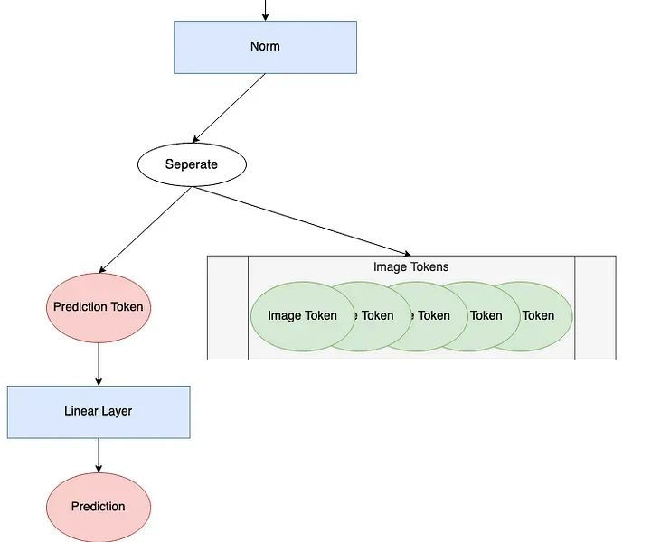
We will look at each step of this process. We will continue using 176 Tokens of length 768. We will use a batch size of 1 to illustrate how to make a single prediction. A batch size greater than 1 will parallelize this prediction.

# Define an Inputnum_tokens = 176token_len = 768batch = 1x = torch.rand(batch, num_tokens, token_len)

<span>print('Input dimensions are

	batchsize:', x.shape[0], '

	number of tokens:', x.shape[1], '

	token length:', x.shape[2])</span>

Input dimensions are batchsize: 1 number of tokens: 176 token length: 768

First, all Tokens are passed through a norm layer.

norm = nn.LayerNorm(token_len)x = norm(x)

<span><span>print</span>(<span>'After norm, dimensions are

	batchsize:'</span>, x.shape[0], <span>'

	number of tokens:'</span>, x.shape[1], <span>'

	token size:'</span>, x.shape[2])</span>

After norm, dimensions are batchsize: 1 number of tokens: 1001 token size: 768

Next, we separate the prediction Token from the remaining Tokens. In the encoding blocks, the prediction Token has become non-zero and has gathered information about our input image. We will use only this prediction Token for the final prediction.

norm = nn.LayerNorm(token_len)pred_token = x[:, 0]print('Length of prediction token:', pred_token.shape[-1])

Length of prediction token: 768

Finally, the prediction Token is passed to the head for prediction. The head is typically some type of neural network, varying depending on the model. In An Image is Worth 16×16 Words², they used an MLP (multi-layer perceptron) with one hidden layer during pre-training and a single linear layer during fine-tuning. In Tokens-to-Token ViT³, they used a single linear layer as the head. This example will use an output shape of 1 to represent a single estimated regression value.

head = nn.Linear(token_len, 1)pred = head(pred_token)print('Length of prediction:', (pred.shape[0], pred.shape[1]))print('Prediction:', float(pred))

Length of prediction: (1, 1)Prediction: -0.5474240779876709

This is all there is to it! The model has made a prediction!

Complete Code

To create the complete ViT module, we use the Patch Tokenization module and ViT Backbone module defined above. The ViT Backbone is defined as follows, containing the Token processing, encoding blocks, and prediction processing components.

class ViT_Backbone(nn.Module):

<span> <span><span>def</span> <span>__init__</span><span>(<span>self</span>,</span></span></span><code><span> <span>preds:</span> int=<span>1</span>,</span>

 token_len: int=768, num_heads: int=1, Encoding_hidden_chan_mul: float=4., depth: int=12, qkv_bias=False, qk_scale=None, act_layer=nn.GELU, norm_layer=nn.LayerNorm): """ VisTransformer Backbone Args: preds (int): number of predictions to output token_len (int): length of a token num_heads(int): number of attention heads in MSA

<span>                Encoding_hidden_chan_mul (float): multiplier to determine the number of hidden channels (features) in the NeuralNet component of the Encoding Module</span>

<span>                norm_layer(nn.modules.normalization): torch neural network layer class to use as normalization</span>

 """""" super().__init__() ## Defining Parameters self.num_heads = num_heads self.Encoding_hidden_chan_mul = Encoding_hidden_chan_mul self.depth = depth ## Defining Token Processing Components

<span> <span>self</span>.cls_token = nn.Parameter(torch.zeros(<span>1</span>, <span>1</span>, <span>self</span>.token_len))</span>

<span> <span>self</span>.pos_embed = nn.Parameter(data=get_sinusoid_encoding(num_tokens=<span>self</span>.num_tokens+<span>1</span>, token_len=<span>self</span>.token_len), requires_grad=False)</span>

 ## Defining Encoding blocks self.blocks = nn.ModuleList([Encoding(dim = self.token_len, num_heads = self.num_heads,

<span>                                               hidden_chan_mul = <span>self</span>.Encoding_hidden_chan_mul,</span>

 qkv_bias = qkv_bias, qk_scale = qk_scale, act_layer = act_layer, norm_layer = norm_layer) for i in range(self.depth)]) ## Defining Prediction Processing self.norm = norm_layer(self.token_len) self.head = nn.Linear(self.token_len, preds) ## Make the class token sampled from a truncated normal distrobution timm.layers.trunc_normal_(self.cls_token, std=.02) def forward(self, x): ## Assumes x is already tokenized ## Get Batch Size B = x.shape[0] ## Concatenate Class Token

<span>        x = torch.cat((<span>self</span>.cls_token.expand(B, -<span>1</span>, -<span>1</span>), x), dim=<span>1</span>)</span>

 ## Add Positional Embedding x = x + self.pos_embed ## Run Through Encoding Blocks for blk in self.blocks: x = blk(x) ## Take Norm x = self.norm(x) ## Make Prediction on Class Token x = self.head(x[:, 0]) return x

Through the ViT Backbone module, we can define the complete ViT model.

class ViT_Model(nn.Module):

<span> <span><span>def</span> <span>__init__</span><span>(self,</span></span></span><code><span>    img_size: tuple[int, int, int]=<span>(<span>1</span>, <span>400</span>, <span>100</span>)</span>,</span>

 patch_size: int=50, token_len: int=768, preds: int=1, num_heads: int=1, Encoding_hidden_chan_mul: float=4., depth: int=12, qkv_bias=False, qk_scale=None, act_layer=nn.GELU, norm_layer=nn.LayerNorm): """ VisTransformer Model Args: img_size (tuple[int, int, int]): size of input (channels, height, width) patch_size (int): the side length of a square patch token_len (int): desired length of an output token preds (int): number of predictions to output num_heads(int): number of attention heads in MSA

<span>    Encoding_hidden_chan_mul (float): multiplier to determine the number of hidden channels (features) in the NeuralNet component of the Encoding Module</span>

 depth (int): number of encoding blocks in the model qkv_bias (bool): determines if the qkv layer learns an addative bias qk_scale (NoneFloat): value to scale the queries and keys by;  if None, queries and keys are scaled by ``head_dim ** -0.5`` act_layer(nn.modules.activation): torch neural network layer class to use as activation norm_layer(nn.modules.normalization): torch neural network layer class to use as normalization """ super().__init__() ## Defining Parameters self.img_size = img_size C, H, W = self.img_size self.patch_size = patch_size self.token_len = token_len self.num_heads = num_heads self.Encoding_hidden_chan_mul = Encoding_hidden_chan_mul self.depth = depth ## Defining Patch Embedding Module self.patch_tokens = Patch_Tokenization(img_size, patch_size, token_len) ## Defining ViT Backbone self.backbone = ViT_Backbone(preds, self.token_len, self.num_heads, self.Encoding_hidden_chan_mul, self.depth, qkv_bias, qk_scale, act_layer, norm_layer) ## Initialize the Weights self.apply(self._init_weights) def _init_weights(self, m): """ Initialize the weights of the linear layers & the layernorms """ ## For Linear Layers if isinstance(m, nn.Linear): ## Weights are initialized from a truncated normal distrobution timm.layers.trunc_normal_(m.weight, std=.02)

<span> <span>if</span> isinstance(m, nn.Linear) <span>and</span> m.bias <span>is</span> <span>not</span> <span>None</span>:</span>

 ## If bias is present, bias is initialized at zero nn.init.constant_(m.bias, 0) ## For Layernorm Layers elif isinstance(m, nn.LayerNorm): ## Weights are initialized at one nn.init.constant_(m.weight, 1.0) ## Bias is initialized at zero nn.init.constant_(m.bias, 0) @torch.jit.ignore ##Tell pytorch to not compile as TorchScript def no_weight_decay(self): """ Used in Optimizer to ignore weight decay in the class token """ return {'cls_token'} def forward(self, x): x = self.patch_tokens(x) x = self.backbone(x) return x

In the ViT model, img_size, patch_size, and token_len define the Patch Tokenization module. They represent the size of the input image, the size of the patches into which it is divided, and the length of the token sequence generated from it. It is through this module that ViT transforms the image into a sequence of tokens that the model can process. num_heads determines the number of “heads” in the multi-head attention mechanism; Encoding_hidden_channel_mul is used to adjust the number of hidden layer channels in the encoding blocks; qkv_bias and qk_scale control the biases and scaling of the query, key, and value vectors, respectively; and act_layer represents the activation function layer, from which we can choose any activation function in torch.nn.modules.activation. Additionally, the depth parameter determines how many such encoding blocks are included in the model.

norm_layer parameter sets the norm inside and outside the encoding block module. It can be chosen from any torch.nn.modules.normalization⁸ layer.

The _init_weights method comes from the T2T-ViT³ code. This method can be used to randomly initialize all learned weights and biases. As implemented, the weights of linear layers are initialized from a truncated normal distribution; the biases of linear layers are initialized to zero; the weights of normalization layers are initialized to one; and the biases of normalization layers are initialized to zero.

Conclusion

Now, we can comprehensively understand how the ViT model works and how to train it!

The GitHub repository for this series of articlesThe GitHub repository for An Image is Worth 16×16 Words²

→ Contains pre-trained models and fine-tuning code; does not include model definitionsViT implemented in PyTorch image models (timm)⁹timm.create_model(‘vit_base_patch16_224’, pretrained=True)

Phil Wang’s vit-pytorch package

Editor / Garvey

Review / Fan Ruiqiang

Verification / Garvey

Click below

Encoding Blocks

Leave a Comment Cancel reply