Understanding Transformer Principles and Implementation in 10 Minutes

Click the above “Visual Learning for Beginners” to select “Star” or “Pin”

Important content delivered at the first time

This article is adapted from | Deep Learning This Little Thing

Models based on Transformer from the paper “Attention Is All You Need” (such as Bert) have achieved revolutionary results in various natural language processing tasks and have replaced RNN as the default option, demonstrating the power of the Transformer.

Here, I will share a method that combines the encoder-decoder architecture with the attention mechanism, based on Harvard’s code “Annotated Transformer”. Code link: The Annotated Transformer.

Table of Contents:

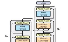
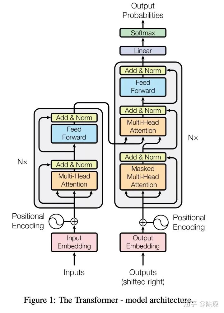
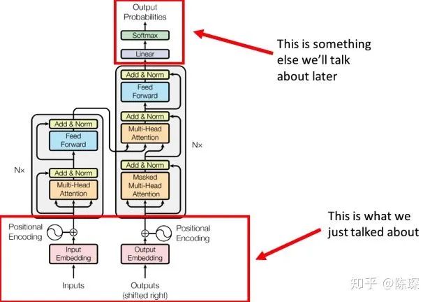
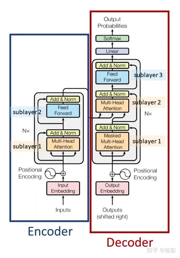
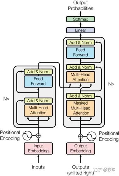
Overall Architecture Description
Input & Output Embedding

OneHot Encoding
Word Embedding
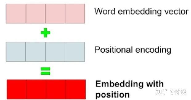
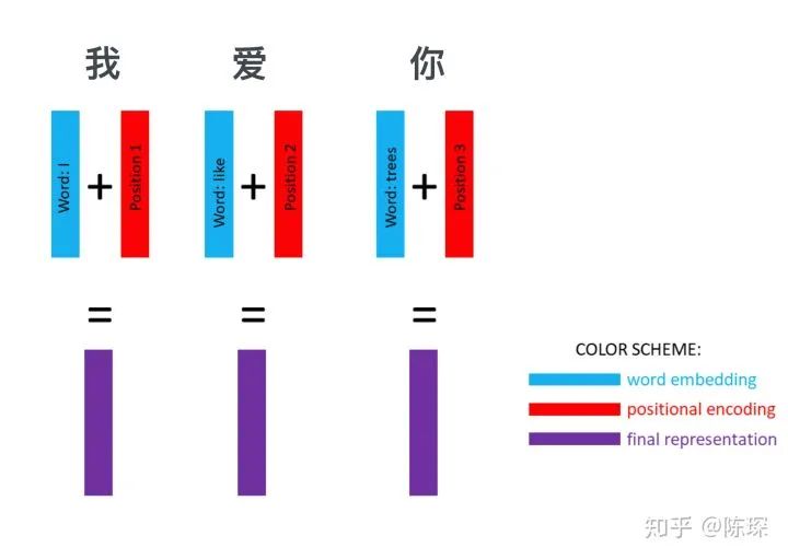
Positional Embedding
Input Short Summary

Encoder

Encoder Sub-layer 1: Multi-Head Attention Mechanism

Step 1
Step 2
Step 3

Encoder Sub-layer 2: Position-Wise Fully Connected Feed-Forward
Encoder Short Summary

Decoder

Diff_1: “masked” Multi-Headed Attention
Diff_2: Encoder-Decoder Multi-Head Attention
Diff_3: Linear and Softmax to Produce Output Probabilities

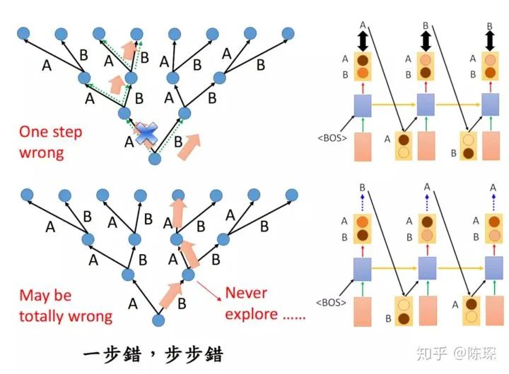
Greedy Search
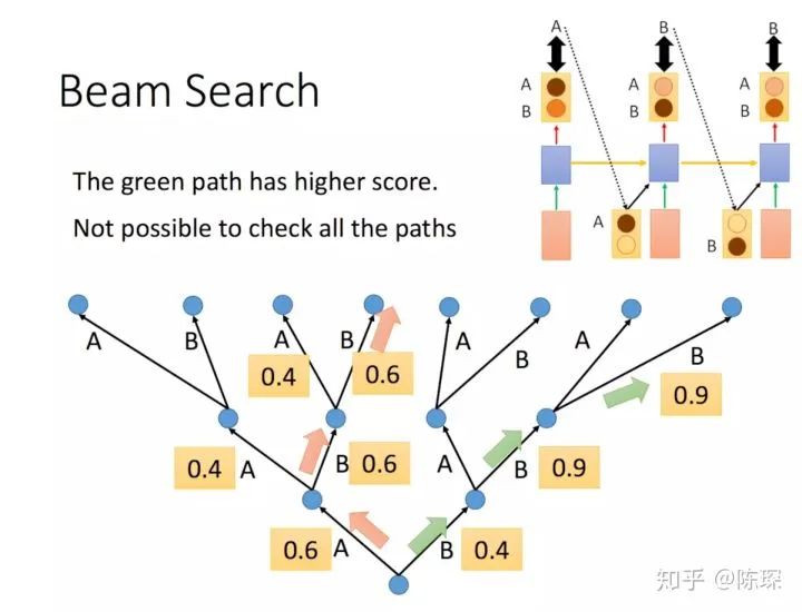
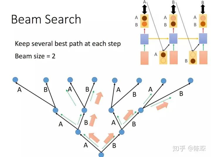
Beam Search
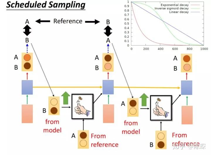
Scheduled Sampling

0. Model Architecture

Understanding Transformer Principles and Implementation in 10 Minutes

Today’s example task is Chinese to English translation: the Chinese input “我爱你” translates to “I Love You” through the Transformer.

Corresponding hyperparameters in the Transformer include:

These are also the hyperparameters used in the function make_model(src_vocab, tgt_vocab, N=6, d_model=512, d_ff=2048, h=8, dropout=0.1).

The entire architecture may seem daunting at first glance, but we need to break down the Transformer for description:

Embedding Part
Encoder Part
Decoder Part

1. Representation of Input and Output

1.1 Representation of Input

First, we use one-hot encoding, a common method for expressing categorical features, to represent the sentence. One-hot means that a vector has only one element as 1, while the rest are 0. Directly, the length of the vector is determined by the vocabulary size. If we want to express 10,000 words, we need a 10,000-dimensional vector.

1.2 Word Embedding

However, we do not directly feed the simple one-hot vector into the Transformer. The reasons include that this representation is very sparse, very large, and cannot express the relationships between words. Therefore, we embed words using shorter vectors to express the attributes of these words. Generally, in Pytorch, we use nn.Embedding, or directly multiply the one-hot vector with a weight matrix W to obtain it.

nn.Embedding contains a weight matrix W, with the corresponding shape of (num_embeddings, embedding_dim). num_embeddings refers to the vocabulary size, i.e., the length of the vocabulary we want to translate. embedding_dim refers to how long the vector used to express a word can be, which can be chosen arbitrarily, such as 64, 128, 256, 512, etc. The Transformer paper chooses 512 (i.e., d_model = 512).

In fact, we can visualize nn.Embedding as a lookup table, where each word has a stored vector. For any given word, we can look up the corresponding result from this table.

There are two options for handling the nn.Embedding weight matrix:

Use pre-trained embeddings and fix them; in this case, it is effectively a lookup table.
Randomly initialize it (of course, we can also choose pre-trained results) but set it to be trainable. This way, we continuously improve the embeddings during the training process.

The Transformer chooses the latter.

In the Annotated Transformer, the class “Embeddings” is used to generate word embeddings, which utilizes nn.Embedding. The specific implementation is as follows:

class Embeddings(nn.Module):
    def __init__(self, d_model, vocab):
        super(Embeddings, self).__init__()
        self.lut = nn.Embedding(vocab, d_model)
        self.d_model = d_model

    def forward(self, x):
        return self.lut(x) * math.sqrt(self.d_model)

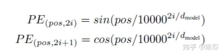
1.3 Positional Embedding

We perform embedding for each word as input representation. However, there is still an issue: the embedding itself does not contain relative position information within the sentence.

Why can RNN use the same vector for the same word anywhere? Because RNN processes the sentence sequentially, one word at a time. However, in the Transformer, all words in the input sentence are processed simultaneously, without considering the order and position information of the words.

To address this, the authors of the Transformer proposed a method to add “positional encoding”. The “positional encoding” allows the Transformer to measure information related to the position of the words.

Adding positional encoding to word embedding yields embedding with position.

So how is “positional encoding” specifically created? How can it express position information? The authors explored two methods for creating positional encoding:

Learn positional encoding vectors through training
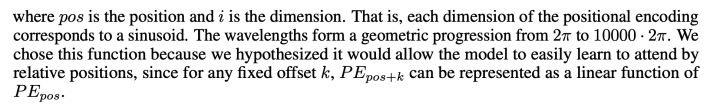
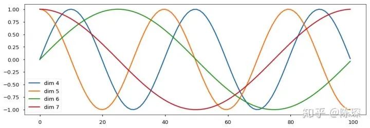
Use formulas to calculate positional encoding vectors

After experiments, it was found that the results of both choices were similar, so the second method was adopted. The advantage is that it does not require training parameters and can be used even for sentence lengths that have not appeared in the training set.

The formula for calculating positional encoding is:

In this formula:

pos refers to the position of the word in the sentence
i refers to the embedding dimension. For example, if d_model=512 is chosen, then i counts from 1 to 512

Why choose sin and cos? Each dimension of the positional encoding corresponds to a sine wave; the authors assume that this allows the model to learn relative positions more easily.

In the Annotated Transformer, the class “Positional Encoding” is used to create positional encoding and add it to the word embedding:

class PositionalEncoding(nn.Module):
    "Implement the PE function."
    def __init__(self, d_model, dropout, max_len=5000):
        super(PositionalEncoding, self).__init__()
        self.dropout = nn.Dropout(p=dropout)

        # Compute the positional encodings once in log space.
        pe = torch.zeros(max_len, d_model)
        position = torch.arange(0, max_len).unsqueeze(1)
        div_term = torch.exp(torch.arange(0, d_model, 2) *
                             -(math.log(10000.0) / d_model))
        pe[:, 0::2] = torch.sin(position * div_term)
        pe[:, 1::2] = torch.cos(position * div_term)
        pe = pe.unsqueeze(0)
        self.register_buffer('pe', pe)

    def forward(self, x):
        x = x + Variable(self.pe[:, :x.size(1)],requires_grad=False)
        return self.dropout(x)

The frequency and offset of the waves are different for each dimension:

1.4 Input Short Summary

After word embedding and positional embedding, we can obtain a representation of a sentence, for example, the sentence “我爱你” is converted into three vectors, each containing the features of the words and their position information in the sentence:

We perform the same operation on the output result, which is the English translation “I Love You”. Using word embedding and positional encoding, we represent it.

The size of the input tensor is [nbatches, L, 512]:

nbatches refers to the defined batch size
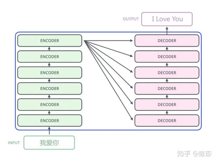
L refers to the length of the sequence (for example, “我爱你”, L = 3)
512 refers to the embedding dimension

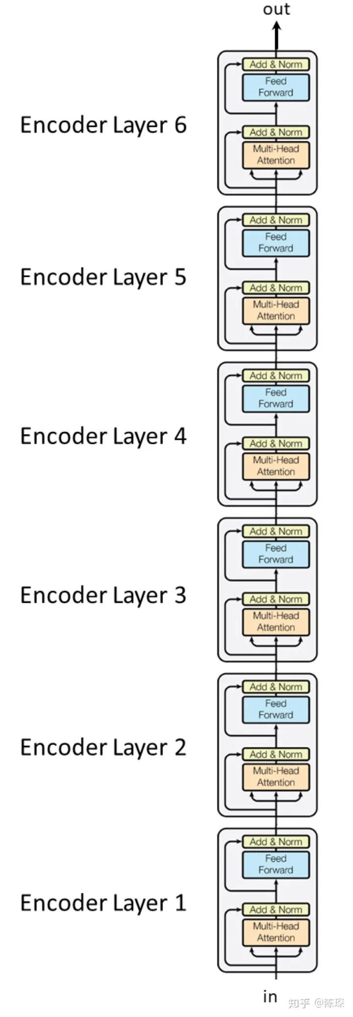
We have now completed the lower-level parts of the model architecture:

2. Encoder

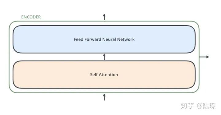
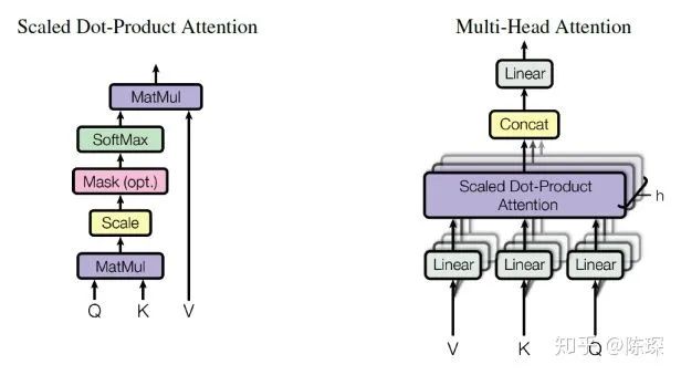
The Encoder is slightly more complicated than the Decoder. The Encoder consists of 6 stacked layers (6 is not fixed and can be modified based on actual conditions), looking like this:

Each layer contains 2 sub-layers:

The first is the “multi-head self-attention mechanism”
The second is a “simple, position-wise fully connected feed-forward network”

The implementation code for the Encoder in the Annotated Transformer is:

class Encoder(nn.Module):
    "Core encoder is a stack of N layers"

    def __init__(self, layer, N):
        super(Encoder, self).__init__()
        self.layers = clones(layer, N)
        self.norm = LayerNorm(layer.size)

    def forward(self, x, mask):
        "Pass the input (and mask) through each layer in turn."
        for layer in self.layers:
            x = layer(x, mask)
        return self.norm(x)

class EncoderLayer(nn.Module):
    "Encoder is made up of self-attn and feed forward (defined below)"
    def __init__(self, size, self_attn, feed_forward, dropout):
        super(EncoderLayer, self).__init__()
        self.self_attn = self_attn
        self.feed_forward = feed_forward
        self.sublayer = clones(SublayerConnection(size, dropout), 2)
        self.size = size

    def forward(self, x, mask):
        "Follow Figure 1 (left) for connections."
        x = self.sublayer[0](x, lambda x: self.self_attn(x, x, x, mask))
        return self.sublayer[1](x, self.feed_forward)

The class “Encoder” stacks <layer> N times, which is an instance of the class “EncoderLayer”.
“EncoderLayer” initialization requires specifying <size>, <self_attn>, <feed_forward>, <dropout>:

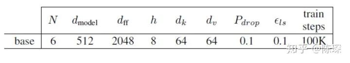
<size> corresponds to d_model, which is 512 in the paper
<self_attn> is an instance of the class MultiHeadedAttention, corresponding to sub-layer 1
<feed_forward> is an instance of the class PositionwiseFeedForward, corresponding to sub-layer 2
<dropout> corresponds to the dropout rate

2.1 Encoder Sub-layer 1: Multi-Head Attention Mechanism

Understanding the Multi-Head Attention mechanism is particularly important for understanding the Transformer, and it is used in both the Encoder and Decoder.

Overview: We define the input to the attention mechanism as x. The meaning of x varies at different positions in the Encoder. At the beginning of the Encoder, x represents the representation of the sentence. In the middle of each layer of the EncoderLayer, x represents the output of the previous EncoderLayer.

Using different linear layers based on x to calculate keys, queries, and values:

key = linear_k(x)
query = linear_q(x)
value = linear_v(x)

linear_k, linear_q, linear_v are independent and have different weights.

After calculating the keys (K), queries (Q), and values (V), the attention is computed using the following formula from the paper:

Matrix multiplication representation:

The strange part here is why do we divide by sqrt(d_k)?

The author’s explanation is to prevent

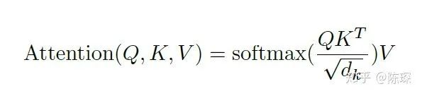
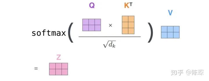
from becoming too large, which would push the softmax function into regions where it has extremely small gradients. The values after applying softmax are between 0 and 1, which can be understood as obtaining attention weights. Then, based on these attention weights, we calculate the weighted sum of V to obtain Attention(Q, K, V).

Detailed explanation: The implementation of Multi-Headed attention in the Annotated Transformer is

class MultiHeadedAttention(nn.Module):
    def __init__(self, h, d_model, dropout=0.1):
        "Take in model size and number of heads."
        super(MultiHeadedAttention, self).__init__()
        assert d_model % h == 0
        # We assume d_v always equals d_k
        self.d_k = d_model // h
        self.h = h
        self.linears = clones(nn.Linear(d_model, d_model), 4)
        self.attn = None
        self.dropout = nn.Dropout(p=dropout)

    def forward(self, query, key, value, mask=None):
        "Implements Figure 2"
        if mask is not None:
            # Same mask applied to all h heads.
            mask = mask.unsqueeze(1)
        nbatches = query.size(0)

        # 1) Do all the linear projections in batch from d_model =&gt; h x d_k
        query, key, value = \
            [l(x).view(nbatches, -1, self.h, self.d_k).transpose(1, 2)
             for l, x in zip(self.linears, (query, key, value))]

        # 2) Apply attention on all the projected vectors in batch.
        x, self.attn = attention(query, key, value, mask=mask,
                                 dropout=self.dropout)

        # 3) "Concat" using a view and apply a final linear.
        x = x.transpose(1, 2).contiguous() \
            .view(nbatches, -1, self.h * self.d_k)
        return self.linears[-1](x)

This class requires specifying:

<h> = 8, which is the number of “heads”. In the base model of the Transformer, there are 8 heads
<d_model> = 512
<dropout> = dropout rate = 0.1

The dimension of keys d_k is calculated based on

. In the above example, d_k = 512 / 8 = 64.

Now let’s detail the forward() function of MultiHeadedAttention in 3 steps:

From the code above, we can see that the forward input includes: query, key, values, and mask. Here we will temporarily ignore the mask. Where do query, key, and value come from? In fact, they are derived from “x” repeated three times, where x can either be the initial sentence embedding or the output of the previous EncoderLayer, as seen in the yellow-highlighted part of the EncoderLayer code, where self.self_attn is an instance of MultiHeadedAttention:

The shape of “query” is [nbatches, L, 512], where:

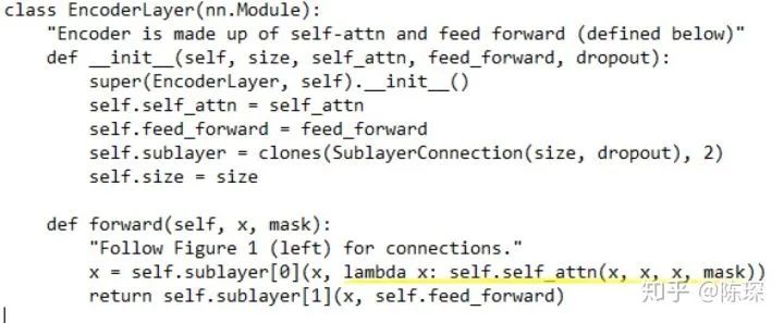
nbatches corresponds to the batch size
L corresponds to the sequence length, where for example, L = 3 for “我爱你”
“key” and “value” also have the shape of [nbatches, L, 512]

Step 1)

Perform linear transformation on “query”, “key”, and “value”; their shape remains [nbatches, L, 512].
Reshape them using view() to the shape of [nbatches, L, 8, 64]. Here, h=8 corresponds to the number of heads, and d_k=64 is the dimension of the keys.
Transpose to swap dimensions 1 and 2, resulting in a shape of [nbatches, 8, L, 64].

Step 2)

As mentioned earlier, we compute the attention using the formula:

The implementation of attention() in the Annotated Transformer is:

def attention(query, key, value, mask=None, dropout=None):
    "Compute 'Scaled Dot Product Attention'"
    d_k = query.size(-1)
    scores = torch.matmul(query, key.transpose(-2, -1)) \
             / math.sqrt(d_k)
    if mask is not None:
        scores = scores.masked_fill(mask == 0, -1e9)
    p_attn = F.softmax(scores, dim = -1)
    if dropout is not None:
        p_attn = dropout(p_attn)
    return torch.matmul(p_attn, value), p_attn

Query and key.transpose(-2,-1) are multiplied, where the shapes are [nbatches, 8, L, 64] and [nbatches, 8, 64, L], respectively. Thus, the resulting scores have the shape of [nbatches, 8, L, L].

After applying softmax to scores, p_attn has the shape of [nbatches, 8, L, L]. The shape of values is [nbatches, 8, L, 64]. Therefore, the final result of multiplying p_attn with values has the shape of [nbatches, 8, L, 64].

In our input and output, there are 8 heads, i.e., the dimension 1 of the tensor is [nbatches, 8, L, 64]. Each of the 8 heads performs different matrix multiplications, resulting in different “representation subspaces”. This is the significance of multi-headed attention.

Step 3)

The initial shape of x is [nbatches, 8, L, 64], and after transposing x.transpose(1,2), we obtain [nbatches, L, 8, 64]. Then, we use view to reshape it to [nbatches, L, 512]. This can be understood as concatenating the results of the 8 heads. Finally, we use the last linear layer for transformation, and the shape remains [nbatches, L, 512], which is exactly the same as the input shape.

For visualization, refer to the diagrams in the paper:

2.2 Encoder Sub-layer 2: Position-Wise Fully Connected Feed-Forward Network

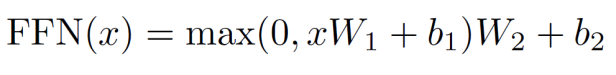
SubLayer-2 is simply a feed-forward network, which is quite straightforward.

The corresponding implementation in the Annotated Transformer is:

class PositionwiseFeedForward(nn.Module):
    "Implements FFN equation."
    def __init__(self, d_model, d_ff, dropout=0.1):
        super(PositionwiseFeedForward, self).__init__()
        self.w_1 = nn.Linear(d_model, d_ff)
        self.w_2 = nn.Linear(d_ff, d_model)
        self.dropout = nn.Dropout(dropout)

    def forward(self, x):
        return self.w_2(self.dropout(F.relu(self.w_1(x))))

2.3 Encoder Short Summary

The Encoder consists of a total of 6 EncoderLayers. Each EncoderLayer contains 2 SubLayers:

SubLayer-1 performs Multi-Headed Attention
SubLayer-2 performs a feedforward neural network

3. The Decoder

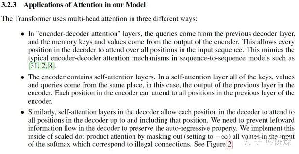
The interaction between the Encoder and Decoder can be understood as:

The Decoder is also a stacked structure of N layers and is divided into 3 SubLayers, highlighting the three main differences between the Encoder and Decoder:

Diff_1: The Decoder SubLayer-1 uses a “masked” Multi-Headed Attention mechanism to prevent the model from seeing the data it is supposed to predict, thus preventing leakage.
Diff_2: SubLayer-2 is an encoder-decoder multi-head attention.
Diff_3: The Linear Layer and Softmax Layer are applied to the output of SubLayer-3 to predict the corresponding word probabilities.

3.1 Diff_1: “masked” Multi-Headed Attention

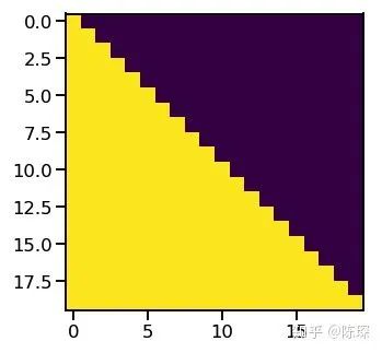
The goal of the mask is to prevent the decoder from “seeing the future”, much like preventing a student from looking at the exam answers. The mask contains 1s and 0s:

The code using the mask in attention is:

if mask is not None:
        scores = scores.masked_fill(mask == 0, -1e9)

As the author stated, “We […] modify the self-attention sub-layer in the decoder stack to prevent positions from attending to subsequent positions. This masking, combined with the fact that the output embeddings are offset by one position, ensures that the predictions for position i can depend only on the known outputs at positions less than i.”

3.2 Diff_2: Encoder-Decoder Multi-Head Attention

The implementation of the DecoderLayer in the Annotated Transformer is:

class DecoderLayer(nn.Module):
    "Decoder is made of self-attn, src-attn, and feed forward (defined below)"
    def __init__(self, size, self_attn, src_attn, feed_forward, dropout):
        super(DecoderLayer, self).__init__()
        self.size = size
        self.self_attn = self_attn
        self.src_attn = src_attn
        self.feed_forward = feed_forward
        self.sublayer = clones(SublayerConnection(size, dropout), 3)

    def forward(self, x, memory, src_mask, tgt_mask):
        m = memory
        x = self.sublayer[0](x, lambda x: self.self_attn(x, x, x, tgt_mask))
        x = self.sublayer[1](x, lambda x: self.src_attn(x, m, m, src_mask))
        return self.sublayer[2](x, self.feed_forward)

The key point is that x = self.sublayer[1] self.src_attn is an instance of MultiHeadedAttention. Here, query = x, key = m, value = m, and mask = src_mask, where x comes from the previous DecoderLayer and m comes from the output of the Encoder.

At this point, we have gathered all three different Attention mechanisms in the Transformer:

3.3 Diff_3: Linear and Softmax to Produce Output Probabilities

The final linear layer expands the output of the decoder to the same dimension as the vocabulary size. After applying softmax, the word with the highest probability is selected as the prediction result.

Assuming we have a trained network, the prediction steps are as follows:

Feed the decoder the embedding result of the entire sentence from the encoder and a special start symbol </s>. The decoder should produce the prediction “I”.
Feed the decoder the embedding result from the encoder and “</s>I”; at this step, the decoder should produce the prediction “Love”.
Feed the decoder the embedding result from the encoder and “</s>I Love”; at this step, the decoder should produce the prediction “China”.
Feed the decoder the embedding result from the encoder and “</s>I Love China”; the decoder should generate the end-of-sentence marker, outputting “</eos>”.
After generating </eos>, the translation is complete.

However, during training, if the decoder is not performing well, the predicted words may not be what we want. If we feed the incorrect data back into the decoder, it will diverge further:

Here, during training, we need to use “teacher forcing”. We utilize the actual word that it should predict at this time and feed it as the correct input.

In addition to selecting the highest word (greedy search), there are other options such as “beam search”, which retains multiple predicted words. The Beam Search method no longer only takes one output to train the next step; we can set a value to take multiple values to train the next step. The probability of this path equals the product of the probabilities of each output step, which can be referenced in the course by Professor Li Hongyi:

Or “Scheduled Sampling”: Initially, we only use the actual sentence sequence for training, and as the training progresses, we gradually start to include the model’s outputs as training inputs.

This part corresponds to the implementation in the Annotated Transformer:

class Generator(nn.Module):
    "Define standard linear + softmax generation step."
    def __init__(self, d_model, vocab):
        super(Generator, self).__init__()
        self.proj = nn.Linear(d_model, vocab)

    def forward(self, x):
        return F.log_softmax(self.proj(x), dim=-1)

Now, let’s review the structure of the Encoder and Decoder with the diagrams:

Reference Links:

https://arxiv.org/pdf/1706.03762.pdf

https://glassboxmedicine.com/2019/08/15/the-transformer-attention-is-all-you-need/

https://jalammar.github.io/illustrated-transformer/

—The End—

Download 1: OpenCV-Contrib Extension Module Chinese Version Tutorial

Reply to “Visual Learning for Beginners” on the WeChat public account:Extension Module Chinese Tutorial to download the first OpenCV extension module tutorial in Chinese, covering more than twenty chapters including extension module installation, SFM algorithms, stereo vision, target tracking, biological vision, super-resolution processing, etc.

Download 2: Python Vision Practical Project 52 Lectures

Reply to “Visual Learning for Beginners” on the WeChat public account:Python Vision Practical Project, to download 31 practical vision projects including image segmentation, mask detection, lane line detection, vehicle counting, eyeliner addition, license plate recognition, character recognition, emotion detection, text content extraction, facial recognition, etc., to help quickly learn computer vision.

Download 3: OpenCV Practical Projects 20 Lectures

Reply to OpenCV Practical Projects 20 Lectures on the WeChat public account: to download 20 practical projects based on OpenCV to advance OpenCV learning.

Group Chat

Welcome to join the public account reader group to communicate with peers. Currently, there are WeChat groups for SLAM, three-dimensional vision, sensors, autonomous driving, computational photography, detection, segmentation, recognition, medical imaging, GAN, algorithm competitions, etc. (will gradually subdivide in the future), please scan the WeChat ID below to join the group, and note: “nickname + school/company + research direction”, for example: “Zhang San + Shanghai Jiao Tong University + Visual SLAM”. Please follow the format; otherwise, you will not be approved. After successfully adding, you will be invited to join the relevant WeChat group based on your research direction. Please do not send advertisements in the group, otherwise you will be removed from the group. Thank you for understanding~