The KNN algorithm is one of the most basic instance-based learning methods. First, we will introduce the relevant concepts of instance-based learning.
1. Instance-Based Learning
1. Given a series of training samples, many learning methods establish a clear generalization description for the objective function; however, instance-based learning methods simply store the training samples.
The work of generalizing from these instances is postponed until a new instance needs to be classified. Whenever the learner encounters a new query instance, it analyzes the relationship between this new instance and the previously stored instances and assigns a value of the objective function to the new instance based on this analysis.
2. Instance-based methods can establish different objective function approximations for different query instances to be classified. In fact, many techniques only establish local approximations of the objective function, applying them to instances that are close to the new query instance, without ever establishing an approximation that performs well across the entire instance space. This approach has significant advantages when the objective function is complex but can be described with less complex local approximations.
3. Limitations of instance-based methods:
(1) The overhead of classifying new instances can be significant. This is because almost all computations occur during classification, not when the training samples are first encountered. Therefore, how to effectively index training samples to reduce the computation required during queries is an important practical issue.
(2) When retrieving similar training samples from memory, they generally consider all attributes of the instances. If the target concept relies only on a few of many attributes, the truly most “similar” instances may be far apart.
2. Principles of the KNN Algorithm
The KNN (k-Nearest Neighbor) algorithm, or K-nearest neighbor algorithm, is arguably one of the easiest classification algorithms to understand in machine learning. As the saying goes: “Birds of a feather flock together.” Indeed, the KNN algorithm is centered around this idea, classifying data accordingly.
K-nearest means that for each sample to be classified, we can classify it based on the majority class of the K nearest sample points. For example, if a new colleague joins the office and the 10 colleagues sitting next to him (K=10) are mostly Python programmers, we would guess that this new colleague is a Python programmer; however, if we expand our judgment to the entire office, assuming there are 50 people (K=50), with 35 being Java programmers, we would conclude that this new colleague is a Java programmer.
Back to the KNN algorithm, the idea and process of classifying data are similar to how we judge a new colleague’s job:
(1) Calculate the distance between the sample to be classified and all known classified samples;
(2) Sort all distances in ascending order;
(3) Take the top K samples;
(4) Count the frequency of each class among the top K samples;
(5) Classify the sample to be classified into the class with the highest frequency.
Now, you should have a basic understanding of the KNN algorithm. However, there are a few questions that need clarification:
-
How to determine the value of K?
-
How to measure distance?
First, let’s discuss how to determine the value of K. The importance of K is evident from the name of the KNN algorithm. Let’s illustrate the importance of K in sample classification with the following example:
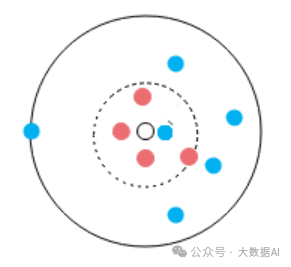
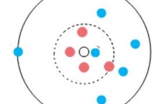
In the figure, all the dots form a dataset, and the color of the dots represents classification. So, which class should the colorless dot belong to?
-
When K=1, the nearest point to the transparent point is the blue dot, so we should classify the transparent dot into the category of the blue dot;
-
When K=5, among the 5 nearest points to the transparent dot, there are 4 red dots and 1 blue dot, so we should classify the transparent dot into the category of the red dots;
-
When K=10, among the 10 nearest points to the transparent dot, there are 4 red dots and 6 blue dots, so we should classify the transparent dot into the category of the blue dots.
As you can see, the final result varies depending on the value of K. A K value that is too large or too small will affect the classification of the data to varying degrees:
When K is small, it means predicting the class of the sample based on nearby samples with small distances, which has the advantage that samples from a farther range do not affect the classification result, resulting in a smaller training error (the error exhibited by a machine learning model on the training dataset is called training error). However, it is prone to overfitting, increasing the generalization error (the expected value of the error exhibited on any test data sample is called generalization error), making the model complex. If there are outliers in the vicinity of the test sample, the classification may be significantly affected. For example, in the above figure, when K=1, if the nearest blue dot is an outlier, then the prediction result for the transparent dot becomes abnormal.
When K is large, it means predicting the class of the test sample based on a larger range of samples, which has the advantage of reducing generalization error, but the training error increases, and the model becomes simpler. An extreme example is when K equals the size of the entire dataset, the entire prediction process becomes of little value, as all test samples will be predicted to belong to the most numerous class in the dataset.
Currently, there is no dedicated theoretical scheme for determining the value of K. A common practice is to divide the dataset into two parts: one part for training and one part for testing. Starting with a small K value, gradually increase K until the highest accuracy is achieved.
Generally, K should not exceed 20, and the upper limit is the square root of n. As the dataset increases, the value of K should also increase. Additionally, K should preferably be an odd number to ensure that the final calculation results in a majority class; using an even number may lead to ties, which is not conducive to prediction.
Regarding distance measurement, the most familiar and widely used is Euclidean distance. The Euclidean distance between two data points in n-dimensional space is defined as:
In addition to Euclidean distance, there are other distance measurement methods such as cosine distance, Hamming distance, Chebyshev distance, etc., but they are less commonly used, so they will not be introduced here.
Finally, let’s summarize the KNN algorithm:
The main advantages of KNN are:
-
Mature theory, simple concept, can be used for both classification and regression
-
Can be used for nonlinear classification
-
Compared to algorithms like Naive Bayes, it makes no assumptions about the data, has high accuracy, and is insensitive to outliers
-
Since the KNN method primarily relies on nearby samples rather than methods that determine class domains, it is more suitable for sample sets with a lot of overlap or crossing class domains
-
This algorithm is particularly suitable for automatic classification of classes with a larger sample size, while using this algorithm for classes with a smaller sample size can easily lead to misclassification
The main disadvantages of KNN are:
-
High computational cost, especially when the number of features is very large
-
When samples are imbalanced, the prediction accuracy for rare classes is low
-
Using lazy learning methods, it does not learn much, resulting in slower prediction speed compared to algorithms like logistic regression
-
Compared to decision tree models, KNN models have weaker interpretability
3. Python Implementation of the KNN Algorithm
KNN classifies by measuring the distances between different feature values. The idea is that if a sample belongs to the majority class among its K most similar (i.e., nearest) samples in feature space, then that sample also belongs to that class. K is usually an integer not greater than 20. In the KNN algorithm, the selected neighbors are all correctly classified objects. This method determines the class of the sample to be classified based only on the classes of the nearest one or several samples.
from numpy import *
import operator


# Given training data and categories
def createDataSet():
    group = array([[1.0, 1.1],
                    [1.0, 1.0],
                    [0, 0],
                    [0, 0.1]])
    labels = ["A", "A", "B", "B"]
    return group, labels


# Classify using KNN
def classify0(inX, dataSet, labels, k):
    # Get the number of rows in the dataset
    dataSetSize = dataSet.shape[0]
    # Calculate Euclidean distance
    # Expand inX to dataSize rows
    diffMat = tile(inX, (dataSetSize, 1)) - dataSet
    sqDiffMat = diffMat ** 2
    sqDistances = sqDiffMat.sum(axis=1)
    distances = sqDistances ** 0.5
    sortedDistIndicies = distances.argsort()
    # Select the smallest k points
    classCount = {}
    for i in range(k):
        voteIlabel = labels[sortedDistIndicies[i]]
        classCount[voteIlabel] = classCount.get(voteIlabel, 0) + 1
    # Decompose classCount dictionary into tuples and sort by the second element in descending order
    sortedClassCount = sorted(classCount.items(), key=operator.itemgetter(1), reverse=True)
    return sortedClassCount[0][0]


if __name__ == '__main__':
    group, labels = createDataSet()
    inX = [0, 0]
    classLabel = classify0(inX, group, labels, 3)
    print(classLabel)
It is recommended to use kd-trees for searching the dataset instead of linear scanning.