
Broadly speaking, NN (or the more elegant DNN) can indeed be considered to encompass specific variants like CNN and RNN. In practical applications, the so-called deep neural network DNN often integrates various known structures, including convolutional layers or LSTM units. However, based on the question posed, the DNN here should specifically refer to a fully connected neural structure, excluding convolutional units or temporal associations.
Therefore, it is entirely reasonable for the questioner to compare DNN, CNN, and RNN. In fact, if we trace the evolution of neural network technology, it becomes easy to understand the original intentions behind the invention of these network structures and their essential differences. Neural network technology originated in the 1950s and 1960s, initially called perceptron, which had an input layer, an output layer, and one hidden layer. The input feature vector is transformed through the hidden layer to reach the output layer, where classification results are obtained.
The early promoter of the perceptron was Rosenblatt. (A tangential note: Due to the limitations of computing technology at the time, the perceptron’s transfer function was mechanically implemented by adjusting resistance using a wire to pull a variable resistor. Just imagine scientists tangled in a mass of wires…) However, Rosenblatt’s single-layer perceptron had a serious flaw: it was incapable of handling even slightly more complex functions (for example, the classic XOR operation).
If it can’t even fit the XOR function, what practical uses can you expect from it? o(╯□╰)o With the advancement of mathematics, this flaw was not overcome until the 1980s by a group of experts including Rumelhart, Williams, Hinton, and LeCun, who invented the multilayer perceptron. A multilayer perceptron, as the name suggests, has multiple hidden layers (obvious, right?). Now, let’s take a look at the structure of a multilayer perceptron:
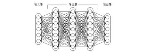
Figure 1: A multilayer perceptron where all neurons in the upper and lower layers are fully connected
The multilayer perceptron can break free from the constraints of early discrete transfer functions, using continuous functions such as sigmoid or tanh to simulate the response of neurons to stimuli, while employing the backpropagation (BP) algorithm invented by Werbos for training.
Yes, this is what we now refer to as neural networks (NN)—neural networks sound so much more advanced than perceptrons! This once again tells us the importance of having a catchy name for research. The multilayer perceptron solved the previous inability to simulate XOR logic, and having more layers allows the network to better model the complexities of the real world.
It’s believed that young Hinton was certainly riding high at that time. The insight brought by the multilayer perceptron is that the number of layers in a neural network directly determines its ability to model reality—using fewer neurons per layer to fit more complex functions [1]. (As Bengio stated: functions that can be compactly represented by a depth k architecture might require an exponential number of computational elements to be represented by a depth k − 1 architecture.)
Even though the experts anticipated that neural networks needed to become deeper, there was always a nightmare lingering. As the number of layers in the neural network increased, the optimization function became increasingly prone to falling into local optima, and this “trap” drifted further away from the true global optimum. Deep networks trained on limited data often performed worse than shallower networks.
Additionally, another issue that cannot be overlooked is that as the number of layers increases, the “vanishing gradient” phenomenon becomes more severe. Specifically, we often use sigmoid as the input-output function for neurons. For a signal with an amplitude of 1, during backpropagation, the gradient decays to 0.25 with each layer it passes through. With many layers, the gradient exponentially decays and the lower layers essentially receive no effective training signal.
In 2006, Hinton alleviated the local optimum problem using a pre-training method, pushing the hidden layers to 7 layers [2], and neural networks truly gained “depth,” thus initiating the wave of deep learning. Here, “depth” does not have a fixed definition—4-layer networks can be considered “deep” in speech recognition, while networks with over 20 layers are common in image recognition.
To overcome the vanishing gradient, functions like ReLU and maxout replaced sigmoid, forming the basic structure of today’s DNN. From a structural standpoint, fully connected DNNs and multilayer perceptrons like in Figure 1 are indistinguishable. Notably, this year’s emergence of highway networks and deep residual learning further mitigated the vanishing gradient problem, achieving unprecedented network depths of over a hundred layers (deep residual learning: 152 layers) [3,4]!
Specific structures can be researched further. If you previously doubted whether many methods were just riding the “deep learning” hype, the results are truly convincing.
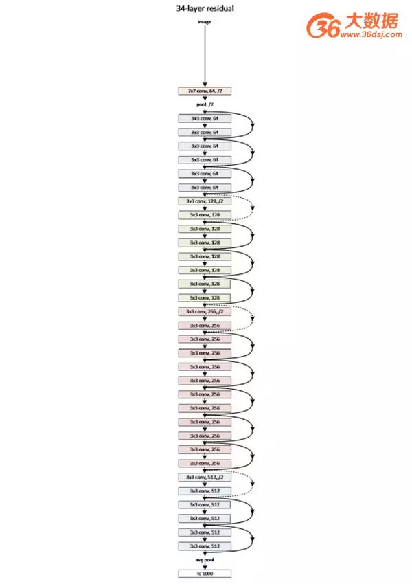
Figure 2: A reduced version of the deep residual learning network, with only 34 layers; the ultimate version has 152 layers
As shown in Figure 1, we see that in the structure of a fully connected DNN, lower layer neurons can connect to all upper layer neurons, leading to a potential problem of parameter explosion. Assuming the input is an image with a resolution of 1K*1K and the hidden layer has 1M nodes, this layer alone would have 10^12 weights to train, which not only makes overfitting likely but also easily leads to local optima.
Moreover, images have inherent local patterns (such as contours, edges, and features like eyes, noses, mouths) that can be utilized; it is clear that the concepts from image processing should be combined with neural network technology. At this point, we can introduce the convolutional neural network (CNN) mentioned by the questioner. In CNNs, not all neurons in adjacent layers can connect directly; instead, they connect via “convolutional kernels” as intermediaries. The same convolutional kernel is shared across all images, and the image retains its original positional relationships after convolution operations.
The illustration of convolutional transmission between two layers is as follows:
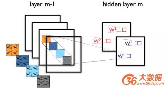
Figure 3: Hidden layer of a convolutional neural network
To briefly explain the structure of a convolutional neural network with an example: Assume that in Figure 3, m-1=1 is the input layer, and we need to recognize a color image that has four channels ARGB (transparency, red, green, and blue, corresponding to four images of the same size). Let’s assume the convolutional kernel size is 100*100, and we use 100 convolutional kernels from w1 to w100 (intuitively, each convolutional kernel should learn different structural features).
Using w1 for convolution operations on the ARGB image can yield the first hidden layer image; the first pixel in the upper left corner of this hidden layer image is the weighted sum of the pixels in the upper left 100*100 area of the four input images, and so on.
Similarly, accounting for other convolutional kernels, the hidden layer corresponds to 100 “images.” Each image responds to different features in the original image. Continuing this structure allows for further transmission. CNNs also include operations like max-pooling to enhance robustness.
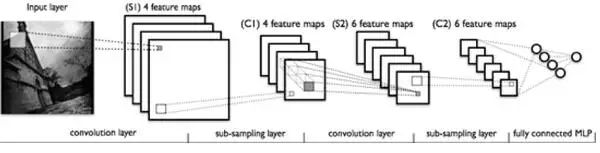
Figure 4: A typical convolutional neural network structure
Note that the last layer is actually a fully connected layer; in this example, we notice that the parameters from the input layer to the hidden layer have instantly reduced to 100*100*100=10^6! This allows us to achieve a good model using the existing training data. The suitability of CNN for image recognition is precisely due to this characteristic of limiting the number of parameters and exploiting local structures. Following the same thought process, using local information from speech spectrograms, CNNs can also be applied in speech recognition.
Fully connected DNNs also face another issue—incapability of modeling changes over time sequences. However, the temporal order of sample occurrence is crucial for applications such as natural language processing, speech recognition, and handwriting recognition. To meet this demand, another type of neural network structure emerged, known as recurrent neural networks (RNN).
In ordinary fully connected networks or CNNs, signals from each layer of neurons can only propagate upwards, and the processing of samples at various time points is independent; hence they are also known as feed-forward neural networks. In RNNs, the output of a neuron can directly affect itself at the next timestamp; that is, the input of the i-th layer neuron at time m includes not only the output of the (i-1)-th layer neuron at that time but also its own output at time (m-1)! This can be illustrated as follows:
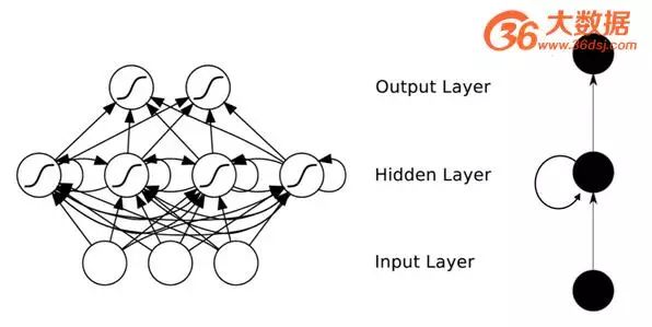
Figure 5: RNN network structure
We can see that interconnections have been added between the hidden layer nodes. For ease of analysis, we often unfold RNNs over time, resulting in the structure shown in Figure 6:
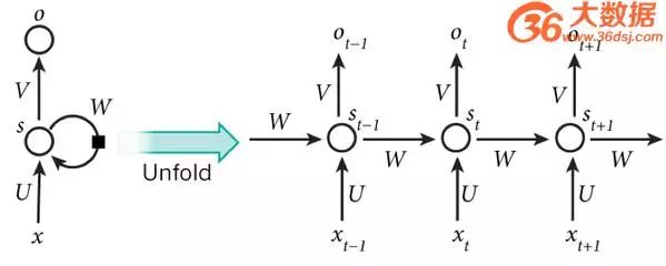
Figure 6: RNN unfolded over time
Cool, the final result O(t+1) of the network at time (t+1) is influenced by the input at that time and all historical inputs! This achieves the goal of modeling time series. Have you noticed, RNN can be seen as a neural network that transmits over time, where its depth is the duration of time! Just as we mentioned earlier, the “vanishing gradient” phenomenon reappears, but this time it occurs along the time axis.
For time t, the gradient it produces vanishes after propagating a few layers back in time, rendering it incapable of affecting the distant past. Therefore, the earlier statement that “all history” collectively influences is merely ideal; in practice, this influence can only last for several timestamps.
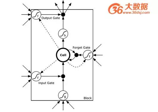
To address the vanishing gradient in time, the machine learning field has developed long short-term memory (LSTM) units, which implement memory functions over time through gate mechanisms and prevent gradient vanishing. An LSTM unit looks like this:
Besides the three networks the questioner is curious about, and the deep residual learning and LSTM I previously mentioned, deep learning encompasses many other structures. For instance, since RNN can inherit historical information, can it also absorb future information?
In sequence signal analysis, if I could foresee the future, it would certainly be helpful for recognition. Hence, bidirectional RNNs and bidirectional LSTMs were developed to utilize both historical and future information.
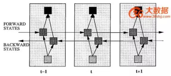
Figure 8: Bidirectional RNN
In fact, regardless of the type of network, they are often used in combination in practical applications. For example, CNNs and RNNs often connect to fully connected layers before the upper layer output, making it difficult to classify a network into a specific category. It is not hard to imagine that as the popularity of deep learning continues, more flexible combinations and various network structures will be developed.
Although it seems ever-changing, researchers’ starting point is undoubtedly to solve specific problems. If the questioner wishes to conduct research in this area, it would be beneficial to analyze the characteristics of these structures and the means by which they achieve their goals.
For beginners, you can refer to:
Ng’s Ufldl: UFLDL Tutorial – Ufldl
You can also check the tutorials included with Theano, which provide very specific examples: Deep Learning Tutorials
Everyone is welcome to continue recommending additional resources.
References:
[1] Bengio Y. Learning Deep Architectures for AI[J]. Foundations & Trends® in Machine Learning, 2009, 2(1):1-127.
[2] Hinton G E, Salakhutdinov R R. Reducing the Dimensionality of Data with Neural Networks[J]. Science, 2006, 313(5786):504-507.
[3] He K, Zhang X, Ren S, Sun J. Deep Residual Learning for Image Recognition. arXiv:1512.03385, 2015.
[4] Srivastava R K, Greff K, Schmidhuber J. Highway networks. arXiv:1505.00387, 2015.

31 Days Until IAIS 2016
November 25-26, China · Optics Valley · East Lake International Conference Center Heavyweight Guests Await!