

This article contains 7196 words, and it is recommended to read in 10 minutes
This article explains how to use TensorFlow for machine learning and deep learning.
1. Introduction
The success of deep learning algorithms has led to groundbreaking advances in artificial intelligence research and applications, greatly changing our lives. More and more developers are learning deep learning development techniques. TensorFlow, launched by Google, is currently the most popular open-source deep learning framework, with rich applications in scenarios such as image classification, audio processing, recommendation systems, and natural language processing. Despite its powerful capabilities, the learning threshold for this framework is not high; as long as you master Python installation and usage, and have some knowledge of machine learning and neural networks, you can get started. This article takes you on an introductory journey into TensorFlow.
2. Getting Started with TensorFlow
2.1. TensorFlow Installation Instructions
Let’s start by installing TensorFlow. TensorFlow is not picky about the environment; it can run on both Python 2.7 and Python 3, and is compatible with operating systems like Linux, MAC, and Windows (note that new versions may initially support only certain operating systems), as long as they are 64-bit. The main difference in installing TensorFlow is that the installation package is available in two versions: one that supports GPU (tensorflow-gpu) and one that does not (tensorflow). It is best to install the GPU-supported version in a production environment to leverage the powerful computing capabilities of the GPU, but this requires the installation of the corresponding CUDA Toolkit and CuDNN first. In contrast, installing the non-GPU version of TensorFlow is easier, and if all goes well, executing the command pip install tensorflow will suffice. If readers encounter issues during installation, they can search online for solutions based on the error messages.
After installation, you can start Python from the command line or open Jupyter Notebook to execute the following command to verify whether TensorFlow has been installed successfully.
>>>import tensorflow as tf
Using tf to reference the TensorFlow package has become a convention. In all the example codes in this article, it is assumed that this statement has been executed beforehand.
2.2. TensorFlow Computational Model
Let’s first see how to compute c = a + b in TensorFlow. Here, a = 3 and b = 2.
>>>a = tf.constant (3)
>>>b = tf.constant (2)
>>>c = a + b
>>>sess = tf.Session ()
>>>print (sess.run(c))
5
From the code above, it can be seen that compared to print (3+2) in Python, achieving the same functionality in TensorFlow requires more steps. First, the parameters need to be packaged and then handed over to the Session object for execution to output the result.
Now, let’s slightly modify the code to let the program output more debugging information.
>>>a = tf.constant (3)
>>>b = tf.constant (2)
>>>print (a, b)
Tensor(“Const:0”, shape=(), dtype=int32) Tensor(“Const_1:0”, shape=(), dtype=int32)
>>>c = a + b
>>>print(c)
Tensor(“add:0”, shape=(), dtype=int32)
>>>sess = tf.Session ()
>>>sess.run ((a,b))
(3,2)
>>>print(sess.run(c))
5
From the above, we can see that a, b, and c are all tensors (Tensor) rather than numbers. The mathematical meaning of a tensor is a multidimensional array. A 1-dimensional array is called a vector, and a 2-dimensional array is called a matrix. Regardless of whether it is 1D, 2D, 3D, or 4D, it can all be referred to as tensors, and even scalars (numbers) can be viewed as 0-dimensional tensors. In deep learning, almost all data can be viewed as tensors, such as the weights and biases of neural networks. A black and white image can be represented as a 2D tensor, where each element represents the grayscale value of a pixel on the image. A color image requires a 3D tensor representation, where two dimensions are width and height, and the other dimension is the color channel. The name TensorFlow contains the word tensor (Tensor). The other word, Flow, means “flow”, representing the expression of computation through the flow of tensors. TensorFlow is a programming system that expresses computation in the form of graphs (Graph), where each node in the graph is an operation (Operation), including computation, initialization, assignment, etc. Tensors are the inputs and outputs of these operations. For example, c = a + b is an addition operation of tensors, which is equivalent to c = tf.add (a, b), where a and b are the inputs to the addition operation, and c is the output of the addition operation.
Submitting the tensor to the session object (Session) for execution yields specific numerical values. In TensorFlow, there are two phases: first, the computation process is defined in the form of a computation graph, and then it is submitted to the session object for execution and returns the computation results. This is because TensorFlow’s core is not implemented in Python, and every function call involves switching between the library and Python, which incurs significant overhead. Moreover, TensorFlow typically runs on GPUs, and if each step is executed automatically, the GPU would waste a lot of resources on repeatedly receiving and returning data, which is far less efficient than receiving and returning data all at once. We can think of TensorFlow’s computation process as ordering takeout. If we dine in at a restaurant, we can eat while the dishes are served. However, if we order takeout, we must first place the entire order at once, then have the other party prepare the food and pack it up, making multiple trips for the delivery impractical.
Equivalently, the statement sess.run (c) can be written as c.eval (session = sess). In terms of objects and parameters, the tensor and session are just swapped. If only one session is used in the context, tf.InteractiveSession() can be used to create a default session object, and subsequent computations do not need to specify it again. That is:
>>>a = tf.constant (3)
>>>b = tf.constant (2)
>>>c = a + b
>>>sess = tf.InteractiveSession ()
>>>print (c.eval())
5
Additionally, in the previous code, the parameters 3 and 2 were hardcoded. If we want to perform the addition operation multiple times, we can replace tf.constant with tf.placeholder, and assign values to the parameters during execution. As shown in the code below:
>>>a = tf.placeholder(tf.int32)
>>>b = tf.placeholder(tf.int32)
>>>c = a + b
>>> sess = tf.InteractiveSession()
# The statement below can also be written as print (sess.run (c, {a:3, b:2}))
>>>print (c.eval ({a:3, b:2}))
5
>>>print (c.eval ({a:[1,2,3], b:[4,5,6]}))
[5 7 9]
Another way to store parameters is to use variable objects (tf.Variable). Unlike tensors created by the tf.constant function, variable objects support parameter updates, but this also means that they rely on more resources and are more tightly bound to sessions. Variable objects must be explicitly initialized within session objects, usually by calling the tf.global_variables_initializer function to initialize all variables at once.
>>>a = tf.Variable (3)
>>>b = tf.Variable (2)
>>>c = a + b
>>>init = tf.global_variables_initializer()
>>>sess = tf.InteractiveSession()
>>>init.run()
>>>print(c.eval())
5
>>>a.load (7)
>>>b.load (8)
>>>print (c.eval())
15
In deep learning, variable objects are often used to represent model parameters that need to be optimized, such as weights and biases, whose values are automatically adjusted during training. This can be seen in later examples in this article.
3. Getting Started with TensorFlow Machine Learning
3.1. Importing Data
MNIST is a very famous handwritten digit recognition dataset, often used as an introductory example for machine learning. TensorFlow’s encapsulation makes using MNIST more convenient. Now we will explore how to use TensorFlow for machine learning using the MNIST digit recognition problem as an example.
MNIST is a collection of images containing 70,000 handwritten digit images:
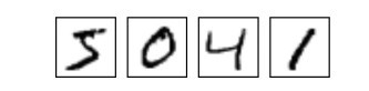
It also includes labels for each image, telling us which digit it represents. For example, the labels for the above four images are 5, 0, 4, and 1, respectively.
In the code below, the input_data.read_data_sets() function downloads and unzips the data.
from tensorflow.examples.tutorials.mnist import input_data
# MNIST_data is a temporary directory for storing data
mnist = input_data.read_data_sets(“MNIST_data/”, one_hot=True)
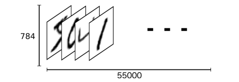
The downloaded dataset is divided into 3 parts: 55,000 training data (mnist.train); 5,000 validation data (mnist.validation); and 10,000 test data (mnist.test). The purpose of this division is to ensure that there is a separate test dataset that is not used for training but is used to evaluate the performance of the model, making it easier to generalize the designed model to other datasets.
Each image contains pixel points. We can represent an image with a numeric array:
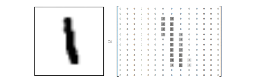
The array is unfolded into a vector of length, so the training dataset mnist.train.images is a tensor with shape [60000, 784]. Each element in this tensor represents the grayscale of a pixel in a certain image, with values ranging between 0 and 1.
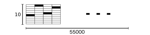
The labels of the MNIST dataset are one-hot vectors of length 10 (because we specified one_hot as True when loading the data). A one-hot vector has all elements as 0 except for one position, which is 1. For example, the label for 3 is represented as ([0, 0, 0, 1, 0, 0, 0, 0, 0, 0]). Therefore, mnist.train.labels is a numerical matrix of shape [55000, 10].
3.2. Designing the Model
Now we will predict the digits in the images by training a machine learning model called Softmax. To recap, classification and regression (numerical prediction) are the two fundamental problems in machine learning. Linear regression is the most basic machine learning model for regression problems, with the basic idea being to assign appropriate weights to various influencing factors, where the predicted result is the weighted sum of these factors. Logistic regression is commonly used for classification problems; it converts results below and above a reference value into values close to 0 and 1, respectively, using the logistic function (also known as the Sigmoid function). However, logistic regression can only handle binary classification problems. Softmax regression is a generalization of logistic regression for multi-class problems. The entire model is illustrated in the figure below:
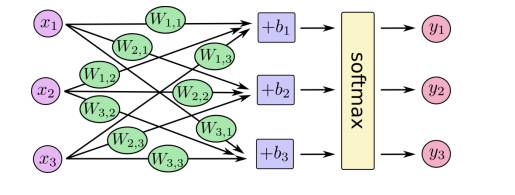
Alternatively, it can be represented using linear algebra formulas:
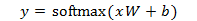
Where x is the feature vector of the input data, with the length of the vector being the number of pixels in the image, and each element in the vector being the grayscale value of each point in the image, W is the weight matrix, where 784 corresponds to the pixels of the image, and 10 corresponds to the digits 0-9. b is a vector of length 10, where each element represents the bias for the digits 0-9, resulting in the weights for each digit, and finally, the softmax function converts the weights into a probability distribution. Typically, we only keep the digit with the highest probability, but sometimes we also pay attention to other digits with relatively high probabilities.
Below is the code to implement this formula in TensorFlow, with the core code being the last statement, where the tf.matmul function indicates matrix multiplication in tensors. Note that slightly different from the formula, here x is declared as a 2D tensor, where the first dimension is of arbitrary length, allowing us to batch process images. Additionally, for simplicity, we use 0 to fill W and b.
x = tf.placeholder (tf.float32, [None, 784])
W = tf.Variable (tf.zeros([784, 10]))
b = tf.Variable (tf.zeros([10]))
y = tf.nn.softmax (tf.matmul (x, W) + b)
In addition to the model, we also need to define a metric to indicate how to optimize the parameters in the model. We typically define a metric to represent the degree to which a model is unsatisfactory and then try to minimize this metric. This metric is called the cost function. The cost function is closely related to the model. Regression problems generally use mean squared error as the cost function, while for classification problems, the commonly used cost function is cross-entropy, defined as
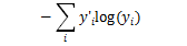
Where y is our predicted probability distribution, and y’ is the actual distribution. Understanding cross-entropy involves knowledge from information theory; here we can think of it as a metric reflecting the mismatch of predictions, or the degree to which the actual situation is unexpected. Note that cross-entropy is asymmetric. In TensorFlow, cross-entropy is represented by the following code:
cross_entropy = -tf.reduce_sum (y_ * tf.log (y))
Since cross-entropy is often used together with Softmax regression, TensorFlow has unified the functions for these two and provided the tf.nn.softmax_cross_entropy_with_logits function. You can directly implement the cross-entropy function after using Softmax regression through the following code. Note that unlike y in the formula, y in the code is the value before calling the Softmax function. Finally, we call tf.reduce_mean to take the average, as a cross-entropy will be calculated for each image in a batch.
y = tf.matmul (x, W) + b
cross_entropy = tf.reduce_mean (
tf.nn.softmax_cross_entropy_with_logits (labels = y_, logits = y))
3.3. Designing the Optimization Algorithm
Now we need to consider how to adjust the parameters to minimize the cost function, which is known as the design problem of the optimization algorithm in machine learning. Here, I will briefly introduce the process of implementing optimization in TensorFlow, as the optimization algorithm is arguably more important than the model itself.
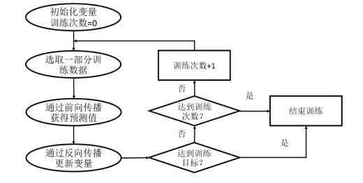
TensorFlow is a deep learning framework based on neural networks. For models like Softmax, they are treated as fully connected neural networks without hidden layers. By adjusting the parameters in the neural network to fit the training data, the model can provide predictive capabilities for unknown samples, manifested as an iterative process of forward propagation and backpropagation. At the beginning of each iteration, we first select all or part of the training data and obtain the prediction results of the neural network model through the forward propagation algorithm. Since the training data are all labeled with correct answers, we can calculate the gap between the predicted answers of the current neural network model and the correct answers. Finally, based on the gap between predicted and true values, the backpropagation algorithm updates the values of the neural network parameters accordingly, making the predictions of the neural network model closer to the true answers on this batch of data. As illustrated in the figure below:
TensorFlow supports various optimizers, and readers can choose different optimization algorithms based on specific applications. The three common optimization methods are tf.train.GradientDescentOptimizer, tf.train.AdamOptimizer, and tf.train.MomentumOptimizer.
train_step = tf.train.GradientDescentOptimizer (0.01).minimize (cross_entropy)
Here, we ask TensorFlow to minimize the cross-entropy using the gradient descent algorithm (Gradient Descent) with a learning rate of 0.01. The gradient descent algorithm is a simple learning process where TensorFlow moves each variable slightly in the direction that continuously lowers the cost. The statement returns train_step, which represents the operation (Operation) to perform optimization, and can be submitted to the session object for execution.
3.4. Training the Model
Now we will start training the model for 1000 iterations. Note that the session object executes not W, b, or y, but train_step.
for i in range(1000):
batch_xs, batch_ys = mnist.train.next_batch(100)
sess.run (train_step, feed_dict = {x: batch_xs, y_: batch_ys})
In each step of this loop, we randomly grab 100 batch data points from the training data, and we use these data points to replace the previous placeholders to run the train_step operation.
Using a small portion of random data for training is called stochastic training – more accurately, stochastic gradient descent training. Ideally, we want to use all our data for every training step, as this would give us better training results, but obviously, this requires a large computational overhead. Therefore, we can use different subsets of data for each training step, which reduces computational overhead while maximizing the learning of the overall characteristics of the dataset.
3.5. Evaluating the Model
It is time to validate whether our model is effective. We can compute y using the trained W and b with the test images and compare the predicted digits with the actual labels of the test images. In Numpy, there is a very useful function argmax, which can give the index of the maximum element in an array. Since the label vector consists of 0s and 1s, the index position of the maximum value of 1 is the category label. For y, the index position of the maximum weight is the predicted digit, as the softmax function is monotonically increasing. The code below compares the predictions of each test image with the actual results and calculates the accuracy using the mean function.
import numpy as np
output = sess.run (y, feed_dict = {x: mnist.test.images})
print (np.mean (np.argmax(output,1) == np.argmax(mnist.test.labels,1)))
We can also let TensorFlow perform the comparison, which is often more convenient and efficient. TensorFlow also has a similar argmax function.
correct_prediction = tf.equal (tf.argmax(y,1), tf.argmax(y_,1))
accuracy = tf.reduce_mean (tf.cast(correct_prediction, “float”))
print (sess.run (accuracy, feed_dict = {x: mnist.test.images, y_: mnist.test.labels}))
The final result should be around 91%. For the complete code, please refer to https://github.com/tensorflow/tensorflow/blob/master/tensorflow/examples/tutorials/mnist/mnist_softmax.py, with minor modifications.
4. Getting Started with TensorFlow Deep Learning
4.1. Introduction to Convolutional Neural Networks
Previously, we used a single-layer neural network. Increasing the number of layers can further improve accuracy. However, increasing the number of layers leads to more parameters to train, which not only slows down computation but also easily causes overfitting. Therefore, a more reasonable neural network structure is needed to effectively reduce the number of parameters in the neural network. For image recognition problems, Convolutional Neural Networks (CNN) are currently the most effective structure.
Convolutional Neural Networks have a hierarchical structure that begins with recognizing pixels and edges, then local shapes, and finally overall perception. In traditional methods, we need to preprocess the images before classification, such as smoothing, denoising, and lighting normalization, from which we extract corner points, gradients, and other features, while Convolutional Neural Networks automate this process. Of course, neural networks are black boxes, and they do not involve the concepts mentioned earlier; they extract abstract features that cannot correspond to the semantic features understood by humans. Moreover, after multiple transformations, the image is unrecognizable. Additionally, Convolutional Neural Networks can be applied beyond image recognition. However, to keep it simple and understandable, we will still use everyday terms like pixels and colors in the following text.
The basic means of feature recognition in Convolutional Neural Networks is convolution. We can understand it as applying special effects to the image, where the pixel value at each position in the new image is a combination or inversion of the pixel values at the corresponding positions and neighboring positions in the original image, similar to filters like blur, sharpen, or mosaic in Photoshop, referred to as filters in TensorFlow. The computation of convolution is the weighted sum of pixels in adjacent areas, expressed in a formula, but the computation is limited to a small rectangular area.
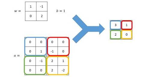
Since convolution only targets adjacent positions in the image, it ensures that after training, there will be the strongest response to local input features. Furthermore, the same set of weights is used regardless of the position in the image, which is equivalent to treating the filter as a flashlight that scans back and forth over the image, ensuring that the content of the image does not affect the judgment. These characteristics of convolutional networks significantly reduce the number of parameters while better utilizing the structural information in the image, extracting features from low-level to complex, and even outperforming human performance.
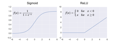
Neural networks need to use activation functions to eliminate linearity; otherwise, even if the depth of the network is increased, it will still be a linear mapping and will not achieve the effect of multiple layers. Unlike the Sigmoid function used in the Softmax model, Convolutional Neural Networks favor the ReLU activation function, which is beneficial for calculations during the backpropagation phase and can alleviate overfitting. The ReLU function is very simple: it ignores outputs less than 0, which can be understood as distinguishing data like folding paper. Note that when using the ReLU function, a good practice is to initialize the bias term with a small positive number to avoid the problem of neuron nodes always outputting 0. The following image compares the Sigmoid and ReLU functions.
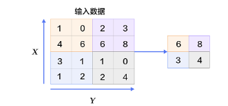
In addition to convolution, Convolutional Neural Networks typically also use downsampling (downsampling or subsampling). We can understand it as appropriately reducing the size of the image, which helps control overfitting to some extent and reduces the impact of image rotation and distortion on feature extraction, as downsampling blurs directional information. Convolutional Neural Networks successfully reduce the high-dimensional image recognition problem through convolution and downsampling, ultimately making it trainable. Downsampling in Convolutional Neural Networks is usually referred to as pooling, which includes max pooling, average pooling, etc. The most common is max pooling, which divides the input data into non-overlapping rectangular regions and takes the maximum value of each rectangular region as output. As shown in the figure below.
4.2. Building the LeNet-5 Network
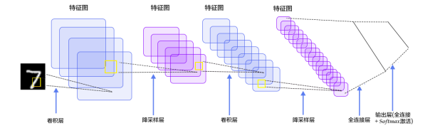
Having gained a basic understanding of Convolutional Neural Networks, we now start using this network to tackle the MNIST digit recognition problem. Here, we refer to the classic LeNet-5 model to introduce how to use TensorFlow for deep learning. The structure of LeNet-5 is illustrated in the figure below. As can be seen, LeNet-5 includes two convolutions and downsampling, followed by two fully connected layers and using Softmax classification as output.
The first layer of the model is the convolutional layer. The input is the original image, with dimensions of, represented in grayscale, and thus the data type is, considering batch input, the data should have 4 dimensions. The filter size is, calculating 32 features, so the weight W is a tensor of, and the bias b is a vector of length 32. Additionally, to ensure that the output image remains the same size, we use 0-padding around the pixels when performing convolution on the edges of the image.
In TensorFlow, the tf.nn.conv2d function implements the algorithm for forward propagation in the convolutional layer. The first two parameters of this function represent the input data x and the weights W, both of which are 4-dimensional tensors, as mentioned earlier. We should add a small amount of noise to the weights during initialization to break symmetry and avoid 0 gradients; here we fill it with random quantities generated by the tf.truncated_normal function. The subsequent two parameters define the method of convolution, including the stride of the filter as it slides over the image and the padding method. The stride is represented by a length-4 array corresponding to the 4 dimensions of the input data; in practice, we only need to adjust the middle two numbers, setting it to [1, 1, 1, 1], which means moving one pixel at a time. The padding can be either “SAME” or “VALID”, where “SAME” means adding full zero padding, while “VALID” means no padding.
The following code implements the first layer of the model:
x = tf.placeholder (tf.float32, [None, 784])
# Here we use the tf.reshape function to correct the dimensions of the tensor, -1 means adaptive
x_image = tf.reshape (x, [-1, 28, 28, 1])
W_conv1 = tf.Variable (tf.truncated_normal ([5, 5, 1, 32], stddev = 0.1))
b_conv1 = tf.Variable (tf.constant (0.1, shape = [32]))
# After executing convolution, use the ReLU function to linearize
h_conv1 = tf.nn.relu (tf.nn.conv2d(
x_image, W_conv1, strides = [1, 1, 1, 1], padding = ‘SAME’) + b_conv1)
The second layer of the model is the downsampling layer. The sampling window size is, non-overlapping, so the stride is also, using max pooling, the size of the image is reduced to half of the original. The function to implement max pooling of the image is tf.nn.max_pool. Its parameters are similar to tf.nn.conv2d, except that the second parameter is not weights but the size of the sampling window, represented by a length-4 array corresponding to the 4 dimensions of the input data.
h_pool1 = tf.nn.max_pool (h_conv1, ksize = [1, 2, 2, 1],
strides = [1, 2, 2, 1], padding = ‘SAME’)
The third layer of the model is a convolutional layer. The input data size is, with 32 features, and the filter size is still, calculating 64 features, so the weight W is of type, and the bias b is a vector of length 64.
W_conv2 = tf.Variable (tf.truncated_normal ([5, 5, 32, 64], stddev = 0.1))
b_conv2 = tf.Variable (tf.constant(0.1, shape = [64]))
# After executing convolution, use the ReLU function to linearize
h_conv2 = tf.nn.relu (tf.nn.conv2d(
h_pool1, W_conv2, strides = [1, 1, 1, 1], padding = ‘SAME’) + b_conv2)
The fourth layer of the model is a downsampling layer, similar to the second layer. The size of the image is again reduced by half.
h_pool2 = tf.nn.max_pool (h_conv2, ksize = [1, 2, 2, 1],
strides = [1, 2, 2, 1], padding = ‘SAME’)
The fifth layer of the model is a fully connected layer. The input data size is, with 64 features, outputting 1024 neurons. Since it is fully connected, both the input data x and the weights W should be 2D tensors. The fully connected parameters are numerous, so we introduce Dropout to prevent overfitting. Dropout randomly disables some weights during each training, averaging the results over multiple training instances while also reducing the coupling between weights. The function to implement Dropout in TensorFlow is tf.nn.dropout. The second parameter of this function indicates the probability that each weight is not disabled.
W_fc1 = tf.Variable (tf.truncated_normal ([7 * 7 * 64, 1024], stddev = 0.1))
b_fc1 = tf.Variable (tf.truncated_normal ([1024], stddev = 0.1))
# Convert 4D tensor to 2D
h_pool2_flat = tf.reshape (h_pool2, [-1, 7*7*64])
h_fc1 = tf.nn.relu (tf.matmul (h_pool2_flat, W_fc1) + b_fc1)
keep_prob = tf.placeholder (tf.float32)
h_fc1_drop = tf.nn.dropout (h_fc1, keep_prob)
The last layer of the model is a fully connected layer plus Softmax output, similar to the previously introduced single-layer model.
W_fc2 = tf.Variable (tf.truncated_normal ([1024, 10], stddev = 0.1))
b_fc2 = tf.Variable (tf.constant(0.1, shape = [10]))
y_conv = tf.matmul (h_fc1_drop, W_fc2) + b_fc2
cross_entropy = tf.reduce_mean(
tf.nn.softmax_cross_entropy_with_logits (labels = y_, logits = y_conv))
4.3. Training and Evaluating the Model
For training and evaluation, we use almost the same set of code as before for the simple single-layer Softmax model, but we will use the more complex ADAM optimizer to shorten the convergence time, and we will also include an additional parameter keep_prob in the feed_dict to control the Dropout ratio. Then we will output a log every 100 iterations.
train_step = tf.train.AdamOptimizer (1e-4).minimize (cross_entropy)
correct_prediction = tf.equal (tf.argmax (y_conv, 1), tf.argmax (y_, 1))
accuracy = tf.reduce_mean (tf.cast (correct_prediction, tf.float32))
sess = tf.InteractiveSession()
sess.run (tf.global_variables_initializer())
for i in range(20000):
batch_xs, batch_ys = mnist.train.next_batch(50)
if i % 100 == 0:
train_accuracy = accuracy.eval (feed_dict = {
x: batch_xs, y_: batch_ys, keep_prob: 1.0})
print(‘step %d, training accuracy %g’ % (i, train_accuracy))
train_step.run (feed_dict = {x: batch_xs, y_: batch_ys, keep_prob: 0.5})
print (‘test accuracy %g’ % accuracy.eval (feed_dict = {
x: mnist.test.images, y_: mnist.test.labels, keep_prob: 1.0}))
The above code should yield an accuracy of approximately 99.2% on the final test set. For the complete code, please refer to https://github.com/tensorflow/tensorflow/blob/master/tensorflow/examples/tutorials/mnist/mnist_deep.py, with some modifications.
5. Conclusion
In this article, we introduced the basic usage of TensorFlow and explained how to use TensorFlow for machine learning and deep learning based on the MNIST data, using both the Softmax model and the Convolutional Neural Network. TensorFlow provides strong support for deep learning, including rich training models, as well as visualization and debugging tools such as TensorBoard, TensorFlow Playground, and TensorFlow Debugger. Due to space limitations, we won’t introduce them all here; please refer to the official TensorFlow documentation for details. Deep learning is a relatively new technology, and there are many pitfalls in both theory and practice. However, as long as you learn and practice more, I believe TensorFlow can become a powerful tool in your hands.
References:
1. “TensorFlow: Practical Google Deep Learning Framework” by Caiyun Technology, Zheng Zeyu, Gu Siyu
2. “TensorFlow Practice for Machine Intelligence” by Sam Abrahams et al., translated by Duan Fei and Chen Peng
3. “Hello, TensorFlow” http://mp.weixin.qq.com/s/0qJmicqIxwS7ChTvIcuJ-g
4. “TensorFlow White Paper” (Translation) http://www.jianshu.com/p/65dc64e4c81f
5. “Convolutional Neural Networks” http://blog.csdn.net/celerychen2009/article/details/8973218
6. “Introduction to Learning Convolutional Neural Networks” http://blog.csdn.net/hjimce/article/details/51761865
Editor: Wen Jing
Author Profile
Wang Xiaojian, Master of Computer Science at Chongqing University, IT veteran, currently engaged in technical research and team management at a company in Chongqing.
He is deeply interested in massive data storage, distributed computing, data analysis, and machine learning, with a focus on performance optimization and natural language processing technologies.
[Review of Previous Articles in the Series]
Exclusive | Understanding Hadoop (I): Overview
Exclusive | Understanding Hadoop (II) HDFS (Part I)
Exclusive | Understanding Hadoop (II) HDFS (Part II)
Exclusive | Understanding Hadoop (III): Mapreduce
Exclusive | Understanding Hadoop (IV): YARN
Exclusive | Understanding Speech Recognition (with Learning Resources)
Exclusive | Understanding Deep Learning (with Learning Resources)
Exclusive | Understanding Transfer Learning (with Learning Toolkit)
Exclusive | Understanding Big Data Processing Frameworks
Exclusive | Understanding Feature Engineering
Exclusive | Understanding Data Visualization
Exclusive | Understanding Clustering Algorithms
Exclusive | Understanding Association Analysis
Exclusive | Understanding Big Data Computing Frameworks and Platforms
Exclusive | Understanding Optical Character Recognition (OCR)
Exclusive | Understanding Regression Analysis
Exclusive | Understanding Non-relational Databases (NoSQL)
Introduction to DataPi Research Department
The DataPi Research Department was established in early 2017, aiming to create a first-class structured knowledge sharing platform and an active community of data science enthusiasts, dedicated to spreading data thinking, enhancing data capabilities, exploring data value, and achieving integration of production, learning, and research!
The logic of the research department lies in knowledge structuring, and practice leads to true knowledge: sorting and building a structured basic knowledge network; original hands-on teaching and practical experience articles; forming professional interest communities for communication and learning, team practice, and tracking the forefront. Interest groups are the core of the research department, each following the overall knowledge sharing and practice project planning of the research department while having its own characteristics: Algorithm Model Group: Actively forming teams to participate in competitions like Kaggle, original hands-on teaching series articles; Research and Analysis Group: Investigating the applications of big data through interviews and exploring the beauty of data products; System Platform Group: Tracking the cutting-edge technology of big data and artificial intelligence system platforms, engaging in conversations with experts; Natural Language Processing Group: Focusing on practice, actively participating in competitions and planning various text analysis projects; Manufacturing Big Data Group: Upholding the dream of becoming an industrial power, integrating production, learning, research, and government, and mining data value; Data Visualization Group: Merging information with art, exploring the beauty of data, and learning to tell stories with visualization; Web Crawling Group: Crawling web information and collaborating with other groups to develop creative projects.
Click on the end of the article “Read the Original” to sign up for DataPi Research Department Volunteers; there’s bound to be a group that suits you~
Note on Reprinting
For reprinting articles, please do the following: 1. Indicate at the beginning of the text: Reprinted from DataPi THU (ID: DatapiTHU); 2. Attach the DataPi QR code at the end of the article.
To apply for reprinting, please send an email to [email protected]