In the previous article, we summarized RNNs (Recurrent Neural Networks). Due to the gradient vanishing problem in RNNs, it is challenging to handle long sequences of data. Experts have improved RNNs, resulting in a special case called LSTM (Long Short-Term Memory), which can avoid the gradient vanishing problem typical of conventional RNNs, thus gaining widespread application in the industry. Below, we will summarize the LSTM model.
Long Short Term Memory networks (hereinafter referred to as LSTMs) are a special type of RNN designed to solve the long dependency problem. This network was introduced by Hochreiter & Schmidhuber (1997) and has been improved and popularized by many. Their work has been used to solve various problems and is still widely applied today.
1. From RNN to LSTM
In the RNN model, we mentioned that RNNs have the following structure, where each sequence index position has a hidden state.
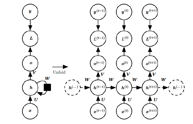
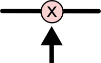
If we omit each layer’s hidden state, the RNN model can be simplified to the following form:
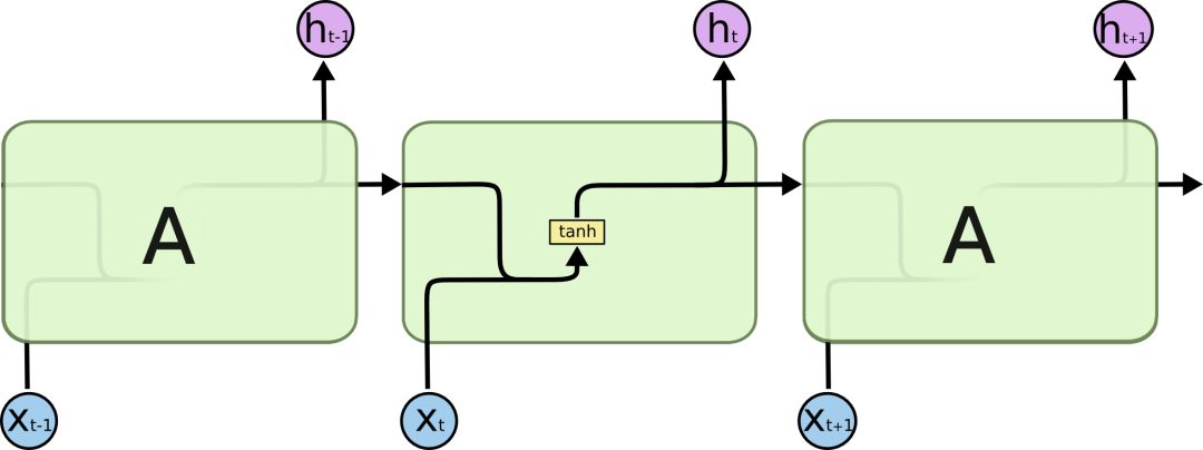
All recurrent neural networks have the form of a chain of repeated modules of neural networks. In standard RNNs, this repeated module has a very simple structure, such as a single tanh layer.
It can be clearly seen in the figure that the hidden state is obtained from and . Due to the gradient vanishing problem in RNNs, experts have improved the hidden structure at the sequence index position, making the hidden structure more complex through some techniques to avoid the gradient vanishing problem. This special RNN is our LSTM.
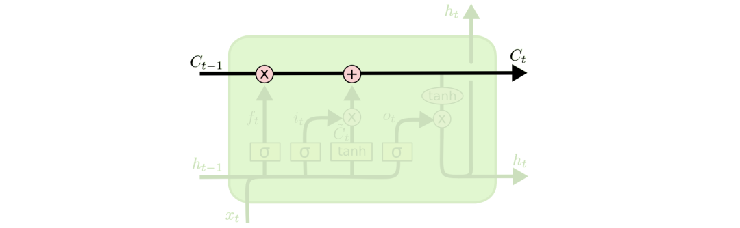
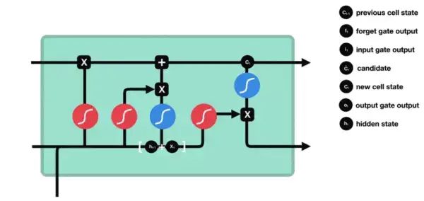
LSTMs also have this chain structure, but their repeating units differ from those in standard RNNs, which only have one network layer; they contain four network layers internally. Since there are many variants of LSTMs, we will discuss the most common LSTM as an example. The structure of LSTMs is shown in the figure below.
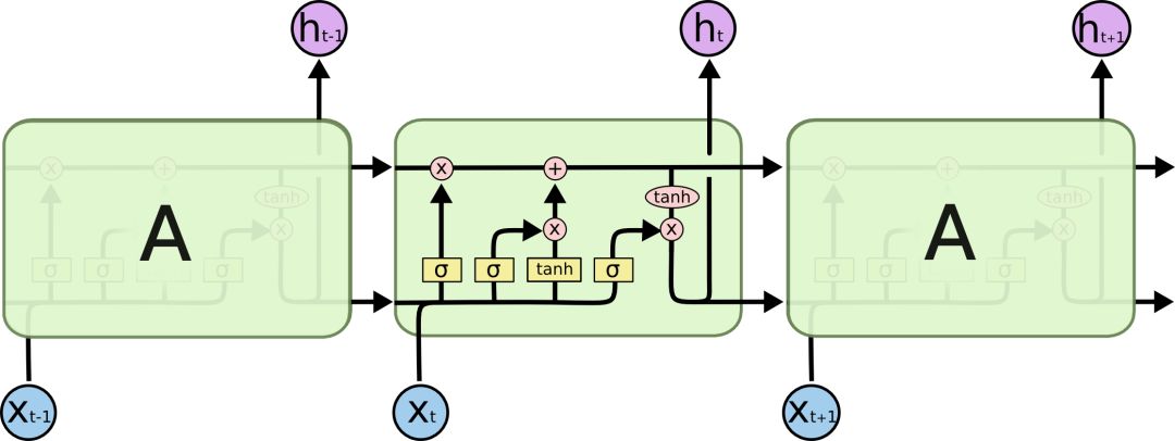
It can be seen that the structure of LSTM is much more complex than that of RNN, and I really admire how experts came up with such a structure that can solve the gradient vanishing problem of RNNs.
When explaining the detailed structure of LSTMs, let’s first define the meanings of various symbols in the figure, which include the following types:
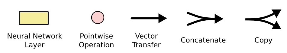
In the above figure, the yellow boxes represent neural network layers, the pink circles indicate point operations such as vector addition and multiplication, single arrows represent data flow direction, arrows merging indicate vector concatenation operations, and arrows branching indicate vector copying operations.
2. Core Ideas of LSTM
The core of LSTMs is the cell state, represented by a horizontal line traversing the unit.
The cell state is somewhat like a conveyor belt. It runs along the entire chain with only some minor linear interactions. Information can flow easily without change. The cell state is shown in the figure below.
LSTMs indeed have the capability to remove or add information to the cell state, carefully regulated by structures called gates.
Gates are a way to selectively allow information to pass through. They consist of a Sigmoid network layer and a pointwise multiplication operation.
Since the output of the sigmoid layer is a value between 0 and 1, it represents how much information can flow through the sigmoid layer. 0 means nothing can pass, while 1 means everything can pass.
An LSTM contains three gates to control the cell state.
3. Understanding LSTM Step by Step
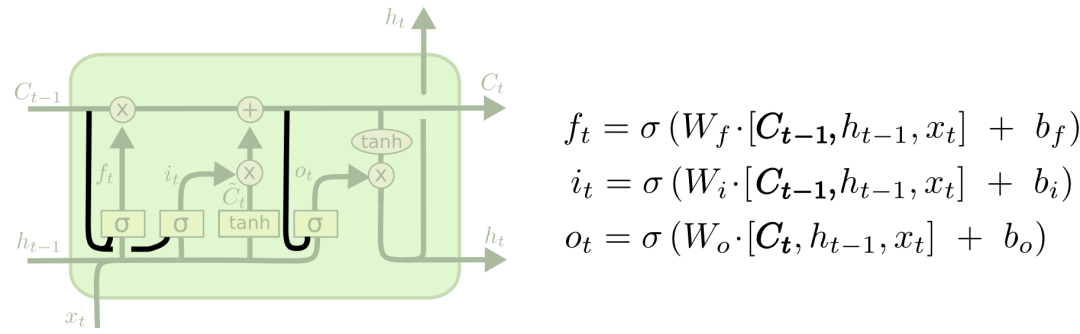
As mentioned earlier, LSTMs control the cell state through three gates, namely the forget gate, input gate, and output gate. Let’s discuss each one.
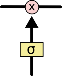
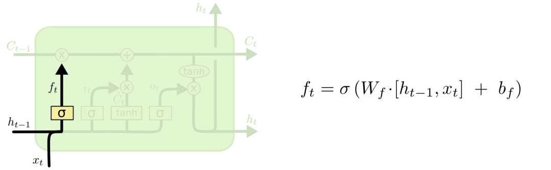
3.1 Forget Gate
The first step of LSTM is to decide which information to discard from the cell state. This operation is handled by a forget gate sigmoid unit. It outputs a vector between 0 and 1 based on the information from and , indicating how much information in the cell state should be retained or discarded. 0 means not retained, and 1 means fully retained. The forget gate is shown in the figure below.
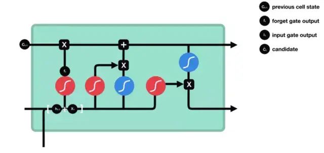
3.2 Input Gate
To update the cell state, we need the input gate. First, we pass the previous hidden state and the current input to the function. This determines which values are updated by transforming them into a range from 0 to 1. 0 means unimportant, and 1 means important. You will also pass the hidden state and the current input to the function, compressing them between -1 and 1 to help regulate the network. Then multiply the output with the output.

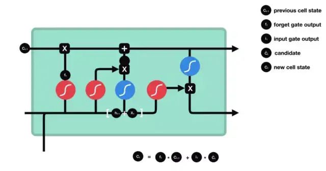
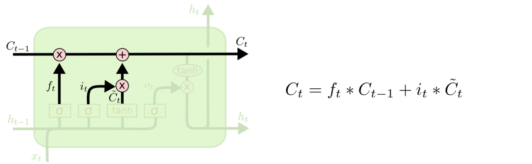
3.3 Cell State
Now we have enough information to calculate the cell state. First, the cell state is pointwise multiplied by the forget vector. If it is multiplied by a value close to 0, it is possible to discard values in the cell state. Then we obtain the output from the input gate and perform pointwise addition to update the cell state with new values that the neural network has found relevant. This results in the new cell state.
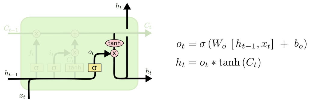
3.4 Output Gate
Finally, we have the output gate. The output gate determines what the next hidden state will be. Remember, the hidden state contains information about previous inputs. The hidden state is also used for prediction. First, we pass the previous hidden state and the current input to the function. Then we pass the new cell state to the function. Multiply the output with the output to determine what information the hidden state should carry. Its output is the hidden state. The new cell state and new hidden state are then passed to the next time step.
The forget gate determines which content is relevant to previous time steps.
The input gate determines which information to add from the current time step.
The output gate determines what the next hidden state should be.
4. Variants of LSTM
The LSTM structure described earlier is the most common. In actual articles, there are various variants of the LSTM structure, although the changes are not significant, they are worth mentioning.
One popular variant proposed by Gers & Schmidhuber (2000) introduces “peephole connections” into the LSTM structure. The role of peephole connections is to allow each gate structure to see cell information, as shown in the figure below.
The above figure adds “peephole connections” to all gates, but many papers only add them to some gates.
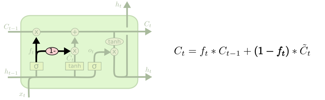
Another variant introduces a coupling between the forget gate and the input gate. Unlike the previous LSTM structure, where the forget gate and input gate are independent, this variant introduces new information at the position where the forget gate removes historical information, deleting old information at the position where new information is added. The structure is shown in the figure below.
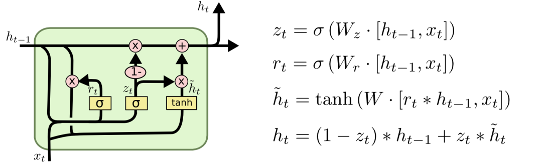
A more significantly different variant of LSTM was proposed by Cho, et al. (2014) called Gated Recurrent Unit (GRU). It merges the forget gate and input gate into a new gate called the update gate. GRU also has a gate called the reset gate. This is shown in the figure below.
5. Conclusion
It has been mentioned that RNNs have achieved good results, many of which are based on LSTMs, indicating that LSTMs are suitable for most sequence scenario applications. Typically, articles will pile up a bunch of formulas to intimidate readers; we hope this step-by-step breakdown can help everyone understand. The use of LSTMs for RNNs is a significant advancement. Now, there is still a question: is there an even greater advancement? For many researchers, the answer is certainly yes, which is the emergence of attention. The idea of attention allows RNNs to select useful information from a larger information set at each step. For example, when using an RNN model to generate letters for an image frame, it will select useful parts of the image to obtain useful input, thereby generating effective output. In fact, Xu, et al. (2015) have already done this; if you want to delve deeper into attention, this would be a great start. There are also some exciting studies in the direction of attention, but much remains to be explored…
6. Reference Links
-
http://colah.github.io/posts/2015-08-Understanding-LSTMs/ -
https://zhuanlan.zhihu.com/p/81549798
