This article will introduce the use of a simple RNN model for time series prediction.
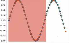
For example, we currently have a segment of a sine curve as shown in the figure below. We will input the red part and train the model to output the next segment’s values.
First, let’s analyze it. Assuming we input 50 points at a time, with the batch size set to 1, each point has one value, so the input shape is [50, 1, 1]. Here, we can represent it differently by placing the batch first, making the shape [1, 50, 1]. This shape can be understood as one curve with a total of 50 points, where each point is a single real number.
import numpy.random import randint
import numpy as np
import torch
from torch import nn, optim
from matplotlib import pyplot as plt
num_time_steps = 50
start = randint(3) # [0, 3)
time_steps = np.linspace(start, start + 10, num_time_steps) # Returns num_time_steps points
data = np.sin(time_steps) # [50]
data = data.reshape(num_time_steps, -1) # [50, 1]
x = torch.tensor(data[:-1]).float().view(1, num_time_steps - 1, 1) # 0~48
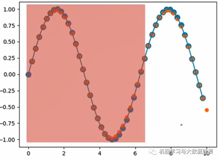
y = torch.tensor(data[1:]).float().view(1, num_time_steps - 1, 1) # 1~49The start variable geometrically represents the value of the x-coordinate corresponding to the left boundary of the red box in the figure, as we need to determine a starting point from which to take 50 points. If this starting point is always the same, the network will memorize it.
x consists of the first 49 data points, which we use to predict one unit of data for each point, and then we compare the results.
Next, we will construct the network architecture.
class Net(nn.Module):
    def __init__(self):
        super(Net, self).__init__()
        self.rnn = nn.RNN(
            input_size=input_size,
            hidden_size=hidden_size,
            num_layers=1,
            batch_first=True,
        )
        self.linear = nn.Linear(hidden_size, output_size)

    def forward(self, x, h0):
        out, h0 = self.rnn(x, h0)  # [b, seq, h] => [seq, h]
        out = out.view(-1, hidden_size)
        out = self.linear(out)  # [seq, h] => [seq, 1]
        out = out.unsqueeze(dim=0)  # => [1, seq, 1]
        return out, h0
First, there is a simple RNN inside, with a parameter batch_first set to True because the format of our data input has the batch first. After the RNN, there is a Linear layer that outputs the memory size as output_size=1 for easy comparison since we only need one value.
Next, we define the training code for the network.
model = Net()
criterion = nn.MSELoss()
optimizer = optim.Adam(model.parameters(), lr)
h0 = torch.zeros(1, 1, hidden_size)  # [b, 1, hidden_size]
for iter in range(6000):
    start = np.random.randint(3, size=1)[0]
    time_steps = np.linspace(start, start + 10, num_time_steps)
    data = np.sin(time_steps)
    data = data.reshape(num_time_steps, 1)
    x = torch.tensor(data[:-1]).float().view(1, num_time_steps - 1, 1)
    y = torch.tensor(data[1:]).float().view(1, num_time_steps - 1, 1)

    output, h0 = model(x, h0)
    h0 = h0.detach()
    loss = criterion(output, y)
    model.zero_grad()
    loss.backward()
    optimizer.step()
    if iter % 100 == 0:
        print("Iteration: {} loss {}".format(iter, loss.item()))
Finally, we will look at the prediction part.
predictions = []
input = x[:, 0, :]
for _ in range(x.shape[1]):
    input = input.view(1, 1, 1)
    (pred, h0) = model(input, h0)
    input = pred
    predictions.append(pred.detach().numpy().ravel()[0])
Assuming the shape of x is [b, seq, 1], after x[:, 0, :], it becomes [b, 1]. However, as mentioned earlier, the batch size is 1, so the input shape is [1, 1]. It is then expanded to [1, 1, 1] to match the network’s input dimensions.
The second to last line and the last line of code do the following: first, the first value is fed in to get an output pred, which is then used as the input for the next prediction, and this process continues, using the last output as the next input.
The final output image is shown below.
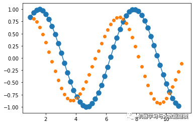
The complete code is as follows:
from numpy.random import randint
import numpy as np
import torch
import torch.nn as nn
import torch.optim as optim
from matplotlib import pyplot as plt

num_time_steps = 50
input_size = 1
hidden_size = 16
output_size = 1
lr=0.01

class Net(nn.Module):
    def __init__(self):
        super(Net, self).__init__()
        self.rnn = nn.RNN(
            input_size=input_size,
            hidden_size=hidden_size,
            num_layers=1,
            batch_first=True,
        )
        self.linear = nn.Linear(hidden_size, output_size)

    def forward(self, x, h0):
        out, h0 = self.rnn(x, h0)  # [b, seq, h]
        out = out.view(-1, hidden_size)
        out = self.linear(out)
        out = out.unsqueeze(dim=0)
        return out, h0

model = Net()
criterion = nn.MSELoss()
optimizer = optim.Adam(model.parameters(), lr)
h0 = torch.zeros(1, 1, hidden_size)
for iter in range(6000):
    start = randint(3)
    time_steps = np.linspace(start, start + 10, num_time_steps)
    data = np.sin(time_steps)
    data = data.reshape(num_time_steps, 1)
    x = torch.tensor(data[:-1]).float().view(1, num_time_steps - 1, 1)
    y = torch.tensor(data[1:]).float().view(1, num_time_steps - 1, 1)

    output, h0 = model(x, h0)
    h0 = h0.detach()
    loss = criterion(output, y)
    model.zero_grad()
    loss.backward()
    optimizer.step()
    if iter % 100 == 0:
        print("Iteration: {} loss {}".format(iter, loss.item()))

start = randint(3)
time_steps = np.linspace(start, start + 10, num_time_steps)
data = np.sin(time_steps)
data = data.reshape(num_time_steps, 1)
x = torch.tensor(data[:-1]).float().view(1, num_time_steps - 1, 1)
y = torch.tensor(data[1:]).float().view(1, num_time_steps - 1, 1)
predictions = []
input = x[:, 0, :]
for _ in range(x.shape[1]):
    input = input.view(1, 1, 1)
    (pred, h0) = model(input, h0)
    input = pred
    predictions.append(pred.detach().numpy().ravel()[0])

x = x.data.numpy().ravel()  # flatten operation
y = y.data.numpy()
plt.scatter(time_steps[:-1], x.ravel(), s=90)
plt.plot(time_steps[:-1], x.ravel())
plt.scatter(time_steps[1:], predictions)
plt.show()
For more articles, you can click on the “Read Original” button below to view.