Recurrent Neural Networks
In traditional neural networks, the model does not pay attention to what information from the previous moment can be used for the next moment; it only focuses on the current moment’s processing. For example, if we want to classify the events that occur at each moment in a movie, knowing the events that happened earlier in the film would make classifying the current moment’s event much easier. In fact, traditional neural networks lack memory functionality, so they do not utilize information from previous moments when classifying events occurring at each moment. So, what method can allow neural networks to remember this information? The answer is Recurrent Neural Networks (RNNs).
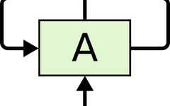
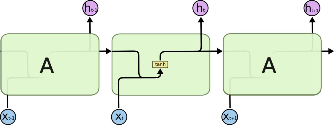
The results of recurrent neural networks differ from traditional neural networks in that they have a loop pointing to themselves, which indicates that they can pass the information processed at the current moment to the next moment. The structure is as follows:
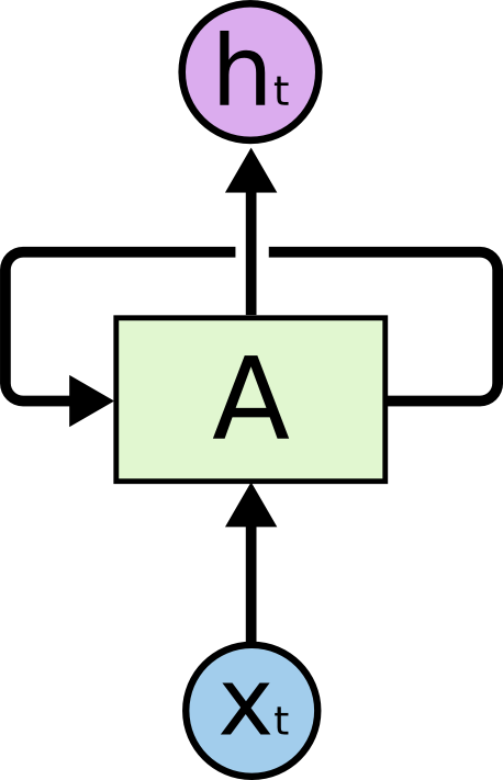
Among them, Xt is the input, A is the model processing part, ht is the output.
To illustrate recurrent neural networks more easily, we expand the above diagram to get:
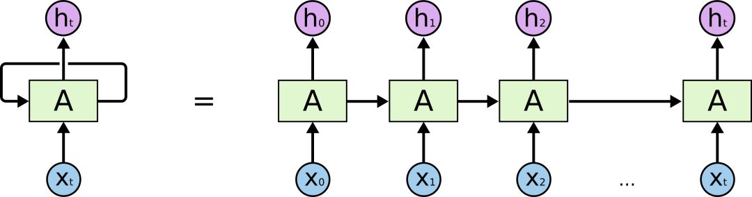
This chain-like neural network represents a recurrent neural network, which can be considered a multiple copy of the same neural network, where the neural network at each moment passes information to the next moment. How do we understand it? Suppose there is a language model, we want to predict the current word based on the words that have appeared in the sentence, the working principle of the recurrent neural network is as follows:
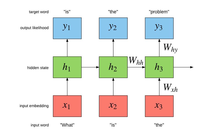
Among them, W represents various weights, x represents input, y represents output, and h represents hidden layer processing state.
Due to its certain memory function, recurrent neural networks can be used to solve many problems, such as: speech recognition, language modeling, machine translation, etc. However, they do not handle long-term dependency problems well.
Long-Term Dependency Problems
Long-term dependency is a problem that arises when the prediction point is far from the relevant information it depends on, making it difficult to learn that relevant information. For example, in the sentence “I was born in France, …, I can speak French”, if we want to predict the end “French”, we need to use the context “France”. Theoretically, recurrent neural networks can handle such problems, but in practice, conventional recurrent neural networks do not solve long-term dependencies well. Fortunately, LSTMs can handle this problem effectively.
LSTM Neural Networks
Long Short Term Memory networks (LSTMs) are a special type of RNNs that can effectively solve long-term dependency problems. So, how do they differ from conventional neural networks? First, let’s take a look at a more specific structure of RNNs:
All recurrent neural networks consist of a chain of repeated neural network modules, and we can see that its processing layer is very simple, usually a single tanh layer, which outputs the current output based on the current input and the output from the previous moment. Compared to neural networks, after a simple modification, it can utilize the information learned from the previous moment for learning at the current moment.
The structure of LSTMs is similar to the above, but the difference is that its repeated modules are somewhat more complex, consisting of four layers:
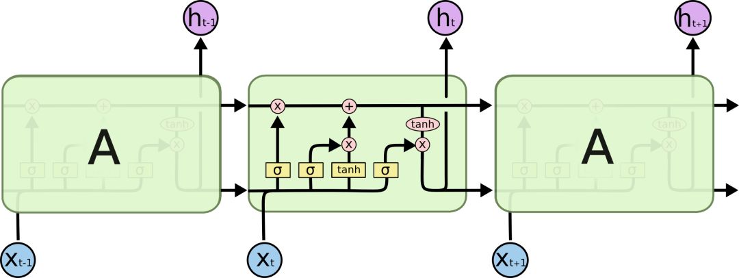
Among them, the symbols and meanings that appear in the processing layer are as follows:
The Core Idea of LSTMs
The key to understanding LSTMs lies in the rectangular box below, known as the memory block, which mainly contains three gates (forget gate, input gate, output gate) and a memory cell. The horizontal line at the top of the box is called the cell state, which acts like a conveyor belt, controlling the information passed to the next moment.

This rectangular box can also be represented as:
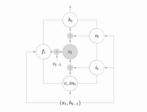
These two diagrams can be viewed together, where the center of the lower diagram, ct is the cell, and the line from the input (ht−1, xt) to the output ht is the cell state. ft, it, ot represent the forget gate, input gate, and output gate, respectively, represented by sigmoid layers. The two tanh layers in the upper diagram correspond to the input and output of the cell.
LSTMs can add and delete information to the cell through gating units. The gates selectively decide whether information should pass through; they consist of a sigmoid neural network layer and a pairwise multiplication operation, as follows:
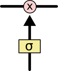
The output of this layer is a number between 0 and 1, indicating how much information is allowed to pass through, where 0 means completely disallowed, and 1 means fully allowed.
Step-by-Step Analysis of LSTM
The first step of LSTM is to determine what information can pass through the cell state. This decision is controlled by the “forget gate” layer through sigmoid, which generates a ft value between 0 and 1 based on the output from the previous moment ht−1 and the current input xt, deciding whether to allow the information learned from the previous moment Ct−1 to pass through or partially pass through. As follows:
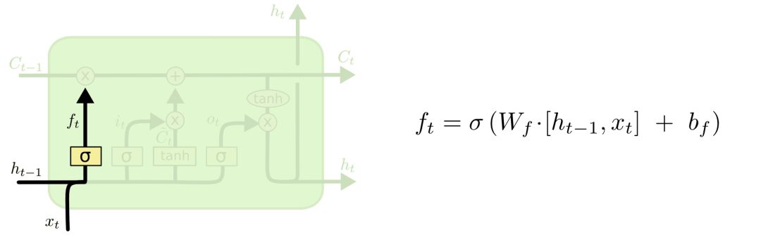
For example, we have learned a lot from the previous sentence, and some of that information is not useful for the current context, so we can selectively filter it out.
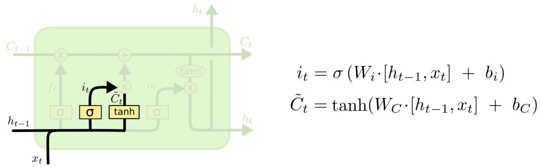
The second step is to generate new information we need to update. This step consists of two parts: the first is an “input gate” layer that uses sigmoid to decide which values to update, and the second is a tanh layer that generates new candidate values C~t, which may be added to the cell state. We will combine the values produced by these two parts for the update.
Now we update the old cell state; first, we multiply the old cell state by ft to forget the information we do not need, then we add it to it∗C~t to get the candidate value.
The combination of the first two steps represents the process of discarding unnecessary information and adding new information:
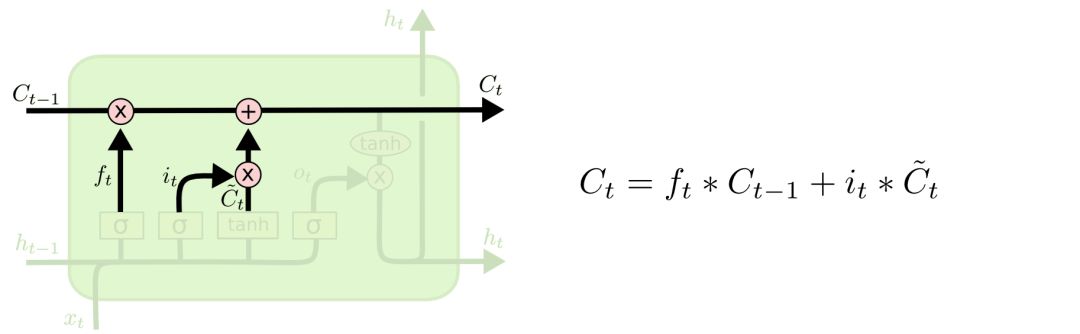
For example, in the previous sentence, we saved the information about Zhang San, and now we have new information about Li Si; we need to discard the information about Zhang San and save the information about Li Si.
The final step is to decide the model’s output; first, we obtain an initial output through the sigmoid layer, then scale the Ct value to between -1 and 1 using tanh, and finally multiply the output obtained from the sigmoid layer to get the model’s output. 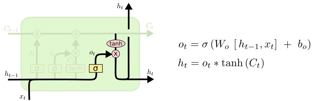
This can be clearly understood; first, the output of the sigmoid function does not consider the information learned from previous moments, while the tanh function compresses and processes the previously learned information, stabilizing the values. The combination of the two is the learning concept of recurrent neural networks. As for how the model learns, that is a process of backpropagation error learning weights.
The above is an understanding of a typical structure of LSTM; of course, it may have some structural variations, but the idea remains basically unchanged, and we will not elaborate further here.
Reference: http://colah.github.io/poss/2015-08-Understanding-LSTMs/
∑ Edited by | Gemini
Source | CSDN Blog

We welcome submissions to the WeChat public account of the beauty of algorithm mathematics.
If the submission involves mathematics, physics, algorithms, computer science, programming, etc., once adopted, we will offer remuneration.
Submission email: [email protected]