
Generative Adversarial Networks (4)

The enthusiastic learner and writer, this yellow duck is back online.
Last time, we discussed the network structure of ACGAN, the method of introducing category information, the metrics for evaluating the performance of generative adversarial networks, methods to improve model training stability, and more.
In the ACGAN paper, there is a statement: “A well-known failure mode of GANs is that the generator will collapse and output a single prototype that maximally fools the discriminator”, meaning that generative adversarial networks often fail due to the generator’s mode collapse (mode collapsing, mode dropping), resulting in the continuous output of the same image that can most effectively deceive the discriminator, leading to extremely poor diversity in generated images.
Aside from mode collapse, another common issue with generative adversarial networks is training instability, which necessitates balancing the training iterations of the generator and discriminator.
Through a series of studies on the GAN objective function, it was found that when the discriminator converges to its optimal point, the objective function equals (-2log(2) + JS divergence). The so-called JS divergence refers to the Jensen-Shannon Divergence. During model training, the value of JS divergence approaches the constant log(2), causing the objective function to approach the constant -log(2). Since the gradient of a constant is zero, when the discriminator converges to its optimal point, the generator’s training will face the problem of gradient vanishing, making it unable to continue.
Regarding the problem of gradient vanishing in the objective function, numerous authors have conducted research. In this article, this yellow duck will introduce LSGAN and WGAN.
First, “Regular GANs adopt the sigmoid cross-entropy loss function for the discriminator. We propose LSGANs which adopt least squares loss function for the discriminator”, meaning that the loss function for the discriminator in other adversarial neural networks is usually cross-entropy, while in LSGAN, the loss function for the discriminator is Least Squares. I know that “Least Squares Method” is the least squares method, so what is “Least Squares”?
Fortunately, the paper’s authors added another sentence: “The idea is to make the generated samples match the statistics of the real data by minimizing the mean square error on an intermediate layer of the discriminator”, indicating that the loss function for the discriminator in LSGAN is mean square error. Although the linear correlation between least squares and mean square error is not very clear, at least this is a concept within my understanding, as the loss function for regression problems often uses mean square error.
The reason for changing the discriminator’s loss function from cross-entropy to mean square error is that when the discriminator converges to its optimal point, the mean square error allows the JS divergence in the objective function to be replaced by the Pearson chi-squared divergence (Pearson χ2 Divergence), thus ensuring that the gradient is not equal to zero, allowing the generator to continue training, making the entire LSGAN training more stable. As for what Pearson chi-squared divergence is, just remember that it is more useful than JS divergence; those interested can explore it further.

Secondly, the quality of images generated by LSGAN is also better than that of other adversarial neural networks. Regarding this point, the authors wrote in the paper: “generate higher quality images”. According to the ACGAN paper, “Quality” has two aspects: one is the accuracy of the discriminator, and the other is the diversity of the generated images. However, the authors of the LSGAN paper did not specify which aspect it referred to, nor did they strictly calculate or compare various metrics. Thus, it can be seen that this conclusion may be drawn empirically, meaning that various experiments were conducted using different neural networks, leading to a general conclusion.
Therefore, understanding the network structure of LSGAN is quite necessary. The authors designed two structures in total. The first one is for inputting images from the LSUN dataset, which consists of five categories. The five categories are “bedroom, kitchen, church, dining room and conference room”, namely bedroom, kitchen, church, dining room, and conference room.
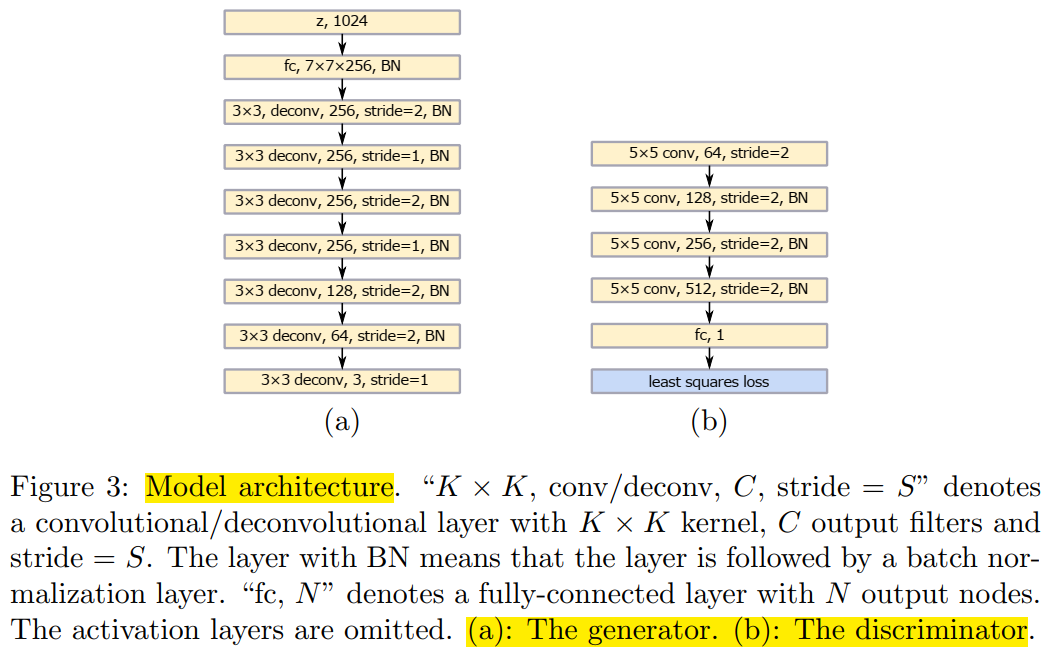
Figure 4-1: The first structure of LSGAN | Source: Paper “Least Squares Generative Adversarial Networks“
Secondly, the second structure is for inputting images belonging to multiple categories, such as Chinese characters. As far as I know, the categories of Chinese characters exceed five, with commonly used characters numbering over two thousand five hundred. In the paper, the number of Chinese characters is set to 3740. If the labels of Chinese character images are converted to integers and then one hot encoding is applied, the result would undoubtedly be a 3740-dimensional sparse matrix.
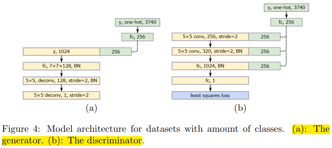
Figure 4-2: The second structure of LSGAN | Source: Paper
From the above images, we can see that both structures of LSGAN are relatively simple. Based on these two images, you should be able to build and train LSGAN.