Top 10 Deep Learning Models

Approximately 10,000 words, recommended reading time: 15 minutes. This article shares the top 10 models in deep learning, which hold significant positions in terms of innovation, application value, and impact.

import tensorflow as tf
from tensorflow.keras.datasets import iris
from tensorflow.keras.models import Sequential
from tensorflow.keras.layers import Dense

# Load the Iris dataset
(x_train, y_train), (x_test, y_test) = iris.load_data()
# Preprocess the data
y_train = tf.keras.utils.to_categorical(y_train)  # Convert labels to one-hot encoding
y_test = tf.keras.utils.to_categorical(y_test)

# Create the neural network model
model = Sequential([
    Dense(64, activation='relu', input_shape=(4,)),  # Input layer with 4 input nodes
    Dense(32, activation='relu'),  # Hidden layer with 32 nodes
    Dense(3, activation='softmax')  # Output layer with 3 nodes (corresponding to 3 types of iris)
])

# Compile the model
model.compile(optimizer='adam',              loss='categorical_crossentropy',              metrics=['accuracy'])

# Train the model
model.fit(x_train, y_train, epochs=10, batch_size=32)

# Test the model
test_loss, test_acc = model.evaluate(x_test, y_test, verbose=2)
print('Test accuracy:', test_acc)

import tensorflow as tf
from tensorflow.keras.models import Sequential
from tensorflow.keras.layers import Conv2D, MaxPooling2D, Flatten, Dense

# Set hyperparameters
input_shape = (28, 28, 1)  # Assume input image is a 28x28 pixel grayscale image
num_classes = 10  # Assume there are 10 classes

# Create CNN model
model = Sequential()
# Add convolutional layer with 32 3x3 filters and ReLU activation function
model.add(Conv2D(32, (3, 3), activation='relu', input_shape=input_shape))
# Add convolutional layer with 64 3x3 filters and ReLU activation function
model.add(Conv2D(64, (3, 3), activation='relu'))
# Add max pooling layer with a 2x2 pooling window
model.add(MaxPooling2D(pool_size=(2, 2)))
# Flatten the multi-dimensional input to one-dimensional for the fully connected layer
model.add(Flatten())
# Add fully connected layer with 128 neurons and ReLU activation function
model.add(Dense(128, activation='relu'))
# Add output layer with 10 neurons and softmax activation function for multi-class classification
model.add(Dense(num_classes, activation='softmax'))
# Compile the model using cross-entropy as the loss function and Adam optimizer
model.compile(loss='categorical_crossentropy', optimizer='adam', metrics=['accuracy'])
# Print model structure
model.summary()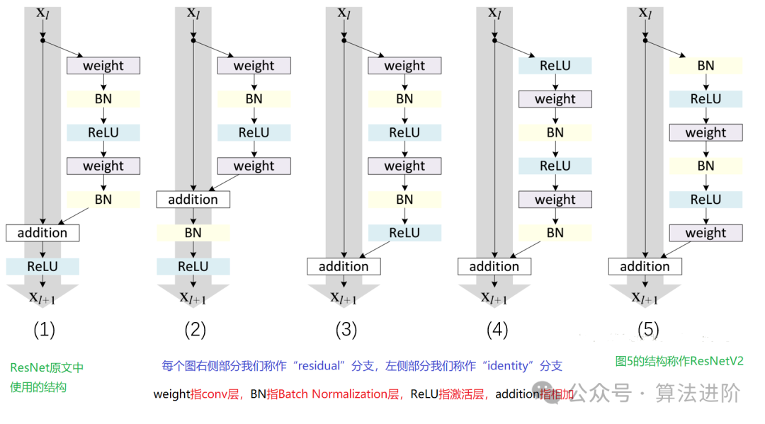

1. Breakthrough in gradient vanishing and model degradation: With the introduction of residual blocks and skip connections, ResNet successfully addresses the training challenges of deep networks, effectively avoiding gradient vanishing and model degradation.
2. Construction of deep network structures: By overcoming the issues of gradient vanishing and model degradation, ResNet is able to build deeper network structures, significantly enhancing model performance.
3. Excellent multi-task performance: Thanks to its powerful feature learning and representation capabilities, ResNet demonstrates outstanding performance across various tasks such as image classification and object detection.

1. High computational resource requirements: Due to the need to construct deep network structures, ResNet requires substantial computational resources and training time.
2. Difficulties in parameter tuning: ResNet has numerous parameters, necessitating significant time and effort for parameter tuning and hyperparameter selection.
3. Sensitivity to initialization weights: ResNet is highly sensitive to the choice of initialization weights; inappropriate initialization may lead to training instability or overfitting issues.

from keras.models import Sequential
from keras.layers import Conv2D, Add, Activation, BatchNormalization

def residual_block(input, filters):
    x = Conv2D(filters=filters, kernel_size=(3, 3), padding='same')(input)
    x = BatchNormalization()(x)
    x = Activation('relu')(x)
    x = Conv2D(filters=filters, kernel_size=(3, 3), padding='same')(x)
    x = BatchNormalization()(x)
    x = Activation('relu')(x)
    return Add()([x, input])  # Add shortcut connection

# Construct ResNet model
model = Sequential()
# Add input layer and other necessary layers
# ...
# Add residual block
model.add(residual_block(previous_layer, filters=64))
# Continue adding more residual blocks and other layers
# ...
# Add output layer
# ...
# Compile and train the model
# model.compile(...)
# model.fit(...)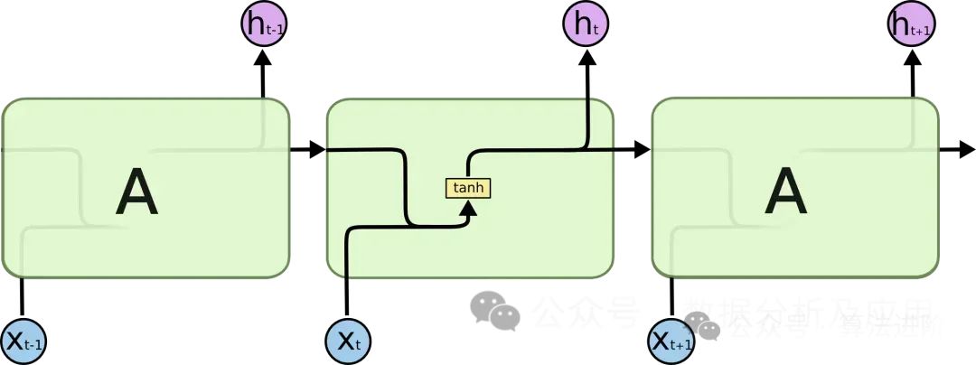

1. Overcoming gradient vanishing and model degradation: By introducing gating mechanisms, LSTM excels in addressing long-term dependency issues, effectively avoiding gradient vanishing and model degradation.
2. Building deep network structures: Thanks to its handling of gradient vanishing and model degradation, LSTM can construct deep and large network structures, fully uncovering the intrinsic patterns of the data and enhancing model performance.
3. Outstanding multi-task performance: LSTM has demonstrated excellent performance across various tasks such as text generation, speech recognition, and machine translation, proving its powerful feature learning and representation capabilities.

1. Challenges in parameter tuning: LSTM involves numerous parameters, making the tuning process cumbersome and requiring significant time and effort for hyperparameter selection and adjustment.
2. Sensitivity to initialization: LSTM is extremely sensitive to the initialization of weights; inappropriate initialization may lead to training instability or overfitting issues.
3. High computational load: Since LSTM typically constructs deep network structures, it requires substantial computational resources and training time.

from keras.models import Sequential
from keras.layers import LSTM, Dense

def lstm_model(input_shape, num_classes):
    model = Sequential()
    model.add(LSTM(units=128, input_shape=input_shape))  # Add an LSTM layer
    model.add(Dense(units=num_classes, activation='softmax'))  # Add a fully connected layer
    return model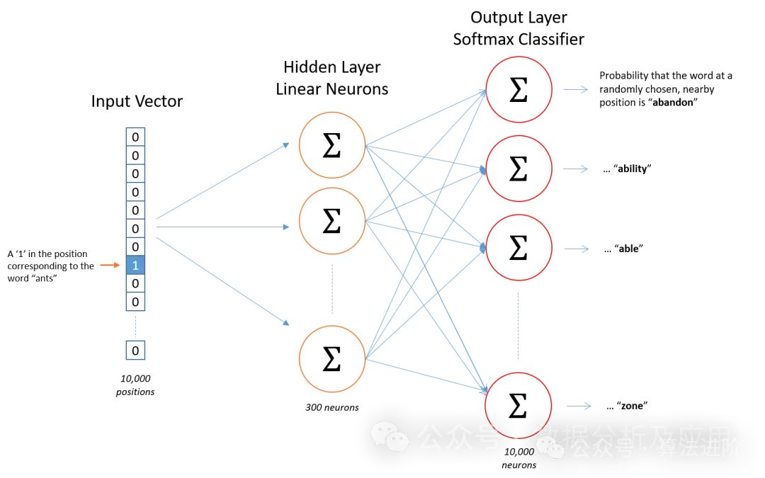

Model Principle

Model Training

Overview of Advantages

1. Semantic similarity: Word2Vec can accurately capture semantic associations between words, bringing semantically similar words closer together in vector space.
2. Training efficiency: The training process of Word2Vec is efficient, easily handling the processing needs of large-scale text data.
3. Interpretability: The word vectors generated by Word2Vec have practical application value and can be used for various tasks such as clustering, classification, and semantic similarity calculations.

Potential Drawbacks

1. Data sparsity: For words that do not appear in the training data, Word2Vec may struggle to generate accurate vector representations.
2. Context window limitations: The fixed context window in Word2Vec may overlook dependencies between words that are far apart.
3. Computational resource demands: The training and inference process of Word2Vec requires certain computational resources.
4. Challenges in parameter tuning: The performance of Word2Vec is highly dependent on the careful tuning of hyperparameters (such as vector dimensions, window sizes, learning rates, etc.).

Application Domains

Python Example Code

from gensim.models import Word2Vec
from nltk.tokenize import word_tokenize
import nltk

# Download punkt tokenizer model
nltk.download('punkt')
# Assume we have some text data
sentences = [
    "I love eating apples",
    "Apples are my favorite",
    "I do not like eating bananas",
    "Bananas are too sweet",
    "I like reading books",
    "Reading makes me happy"
]
# Tokenize the text data
sentences = [word_tokenize(sentence) for sentence in sentences]
# Create Word2Vec model
# The parameters here can be adjusted as needed
model = Word2Vec(sentences, vector_size=100, window=5, min_count=1, workers=4)
# Train the model
model.train(sentences, total_examples=model.corpus_count, epochs=10)
# Get word vector
vector = model.wv['apple']
# Find the most similar words to "apple"
similar_words = model.wv.most_similar('apple')
print("Word vector for apple:", vector)
print("Words similar to apple:", similar_words)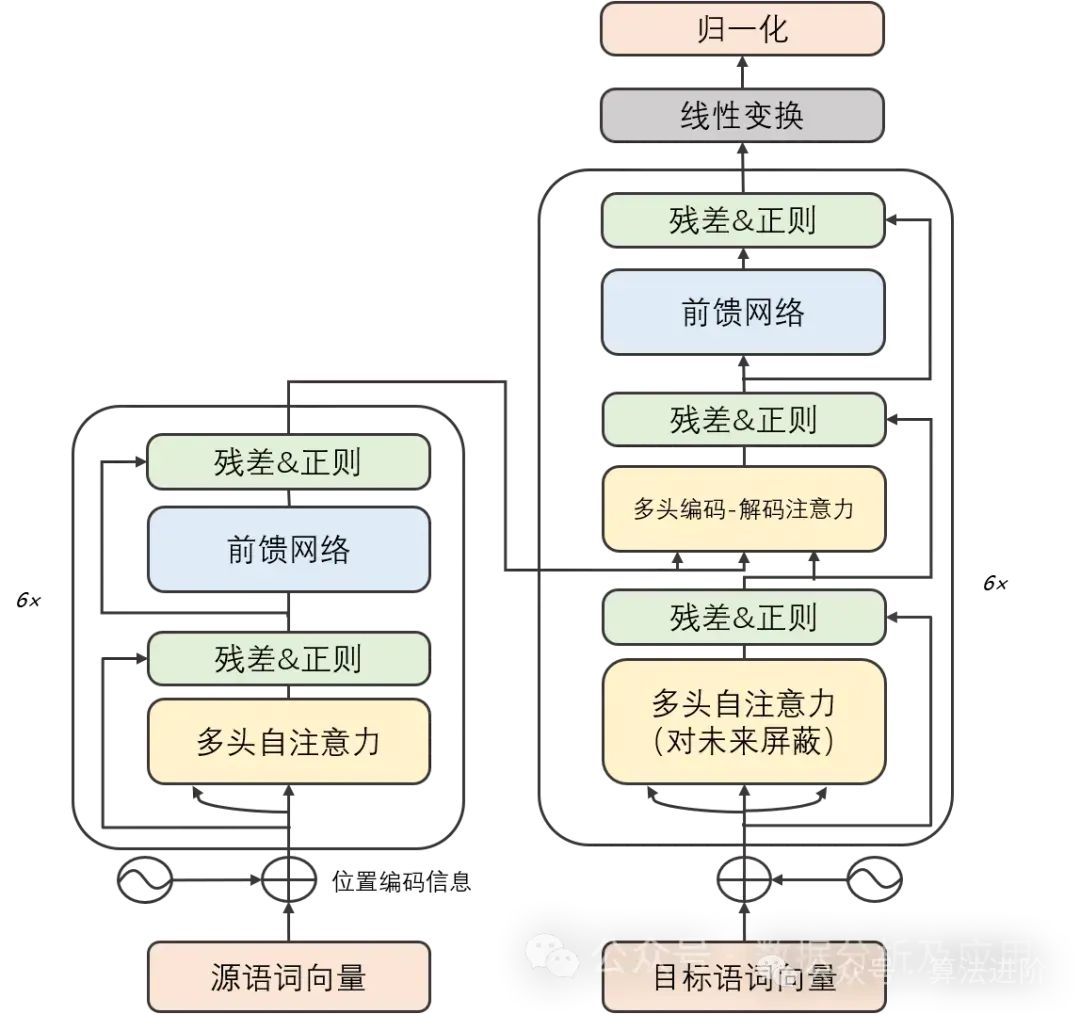

1. Solving the issues of gradient vanishing and model degradation: The Transformer model, with its unique self-attention mechanism, adeptly captures long-term dependencies in sequences, freeing itself from the shackles of gradient vanishing and model degradation.
2. Exceptional parallel computing capabilities: The computational architecture of the Transformer model possesses inherent parallelism, allowing for rapid training and inference on GPUs.
3. Outstanding multi-task performance: With its powerful feature learning and representation capabilities, the Transformer model demonstrates exceptional performance across multiple tasks such as machine translation, text classification, and speech recognition.

1. High computational resource requirements: Due to the computational parallelism of the Transformer model, both training and inference processes require substantial computational resources.
2. Sensitivity to initialization weights: The Transformer model is extremely picky about the choice of initialization weights; improper initialization may lead to training instability or overfitting issues.
3. Limitations in handling long-term dependencies: Although the Transformer model effectively addresses gradient vanishing and model degradation issues, it still faces challenges when processing ultra-long sequences.

import torch
import torch.nn as nn
import torch.optim as optim

# This example is only for illustrating the basic structure and principles of the Transformer. Actual Transformer models (like GPT or BERT) are much more complex and require additional preprocessing steps such as tokenization, padding, masking, etc.
class Transformer(nn.Module):
    def __init__(self, d_model, nhead, num_encoder_layers, num_decoder_layers, dim_feedforward=2048):
        super(Transformer, self).__init__()
        self.model_type = 'Transformer'
        # Encoder layers
        self.src_mask = None
        self.pos_encoder = PositionalEncoding(d_model, max_len=5000)
        encoder_layers = nn.TransformerEncoderLayer(d_model, nhead, dim_feedforward)
        self.transformer_encoder = nn.TransformerEncoder(encoder_layers, num_encoder_layers)
        # Decoder layers
        decoder_layers = nn.TransformerDecoderLayer(d_model, nhead, dim_feedforward)
        self.transformer_decoder = nn.TransformerDecoder(decoder_layers, num_decoder_layers)
        # Decoder
        self.decoder = nn.Linear(d_model, d_model)
        self.init_weights()

    def init_weights(self):
        initrange = 0.1
        self.decoder.weight.data.uniform_(-initrange, initrange)

    def forward(self, src, tgt, teacher_forcing_ratio=0.5):
        batch_size = tgt.size(0)
        tgt_len = tgt.size(1)
        tgt_vocab_size = self.decoder.out_features
        # Forward pass through encoder
        src = self.pos_encoder(src)
        output = self.transformer_encoder(src)
        # Prepare decoder input with teacher forcing
        target_input = tgt[:, :-1].contiguous()
        target_input = target_input.view(batch_size * tgt_len, -1)
        target_input = torch.autograd.Variable(target_input)
        # Forward pass through decoder
        output2 = self.transformer_decoder(target_input, output)
        output2 = output2.view(batch_size, tgt_len, -1)
        # Generate predictions
        prediction = self.decoder(output2)
        prediction = prediction.view(batch_size * tgt_len, tgt_vocab_size)
        return prediction[:, -1], prediction

class PositionalEncoding(nn.Module):
    def __init__(self, d_model, max_len=5000):
        super(PositionalEncoding, self).__init__()
        # Compute the positional encodings once in log space.
        pe = torch.zeros(max_len, d_model)
        position = torch.arange(0, max_len).unsqueeze(1).float()
        div_term = torch.exp(torch.arange(0, d_model, 2).float() * -(torch.log(torch.tensor(10000.0)) / d_model))
        pe[:, 0::2] = torch.sin(position * div_term)
        pe[:, 1::2] = torch.cos(position * div_term)
        pe = pe.unsqueeze(0)
        self.register_buffer('pe', pe)

    def forward(self, x):
        x = x + self.pe[:, :x.size(1)]
        return x

# Hyperparameters
d_model = 512
nhead = 8
num_encoder_layers = 6
num_decoder_layers = 6
dim_feedforward = 2048
# Instantiate model
model = Transformer(d_model, nhead, num_encoder_layers, num_decoder_layers, dim_feedforward)
# Randomly generate data
src = torch.randn(10, 32, 512)
tgt = torch.randn(10, 32, 512)
# Forward pass
prediction, predictions = model(src, tgt)
print(prediction)

7. Generative Adversarial Network (GAN)

The idea of GAN originates from the zero-sum game in game theory, where one player attempts to generate the most realistic fake data, while the other player tries to distinguish between real and fake data. GAN evolved from the Monty Hall problem (a problem combining generative and discriminative models), but unlike the Monty Hall problem, GAN does not emphasize approximating certain probability distributions or generating specific samples; instead, it directly utilizes generative models and discriminative models in an adversarial manner.

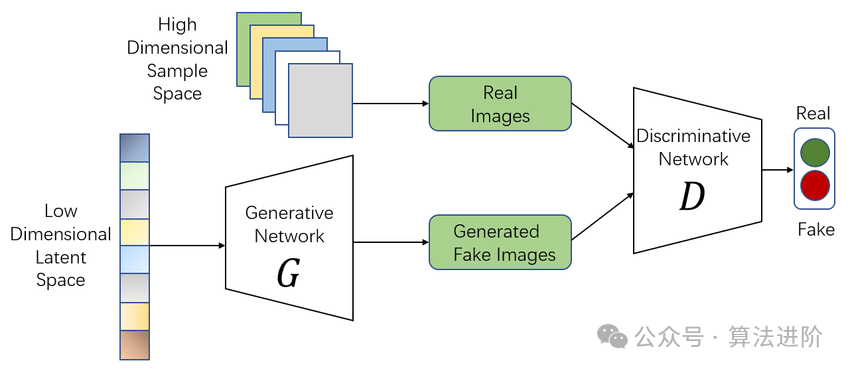
Model Principle: GAN consists of two parts: the generator and the discriminator. The generator is dedicated to creating realistic fake data, while the discriminator aims to distinguish the authenticity of the input data. In a continuous game, both continuously adjust their parameters until they reach a dynamic equilibrium. At this point, the fake data generated by the generator is so realistic that the discriminator finds it challenging to discern its authenticity.

Model Training:

The training process of GAN is a delicate optimization process. In each training step, the generator first generates fake data using current parameters, and the discriminator subsequently judges the authenticity of this data. Based on the discrimination results, the discriminator’s parameters are updated. Simultaneously, to prevent the discriminator from becoming overly precise, we also train the generator to produce fake data that can deceive the discriminator. This process is repeated until both parties reach a subtle balance.

Advantages:

1. Powerful generative capability: GAN can deeply explore the intrinsic structure and distribution patterns of data, creating extremely realistic fake data.

2. No explicit supervision required: During the training process of GAN, there is no need to provide explicit label information; only real data is needed.

3. High flexibility: GAN can seamlessly integrate with other models, such as combining with autoencoders to form AutoGAN or with convolutional neural networks to form DCGAN, thereby expanding its application scope.

Disadvantages:

1. Unstable training: The training process of GAN can be challenging, sometimes leading to mode collapse, where the generator focuses solely on generating a specific type of sample, making it difficult for the discriminator to judge accurately.

2. Debugging difficulties: The interactivity between the generator and discriminator is complex, making debugging GAN quite challenging.

3. Evaluation challenges: Given GAN’s excellent generative capability, accurately assessing the authenticity and diversity of the generated fake data is not an easy task.

Use Cases:

1. Image generation: GAN shines in the field of image generation, capable of creating images in various styles, such as generating images based on textual descriptions or transforming one image into another style.

2. Data augmentation: GAN can generate fake data that closely resembles real data, used to expand datasets or enhance the generalization ability of models.

3. Image restoration: With GAN, we can repair defects in images or eliminate noise from images, significantly improving image quality.

4. Video generation: GAN-based video generation has become one of the current research hotspots, capable of creating uniquely styled video content.

Simple Python Example Code:

Below is a simple GAN example code implemented using PyTorch:

import torch
import torch.nn as nn
import torch.optim as optim
import torch.nn.functional as F

# Define the generator and discriminator network structures
class Generator(nn.Module):
    def __init__(self, input_dim, output_dim):
        super(Generator, self).__init__()
        self.model = nn.Sequential(
            nn.Linear(input_dim, 128),
            nn.ReLU(),
            nn.Linear(128, output_dim),
            nn.Sigmoid()
        )

    def forward(self, x):
        return self.model(x)

class Discriminator(nn.Module):
    def __init__(self, input_dim):
        super(Discriminator, self).__init__()
        self.model = nn.Sequential(
            nn.Linear(input_dim, 128),
            nn.ReLU(),
            nn.Linear(128, 1),
            nn.Sigmoid()
        )

    def forward(self, x):
        return self.model(x)

# Instantiate the generator and discriminator objects
input_dim = 100  # Input dimension can be adjusted as needed
output_dim = 784  # For the MNIST dataset, output dimension is 28*28=784
gen = Generator(input_dim, output_dim)
disc = Discriminator(output_dim)

# Define the loss function and optimizer
criterion = nn.BCELoss()  # Binary cross-entropy loss suitable for the GAN's discriminator and generator
# ... (additional training code would go here)

8. Diffusion Model

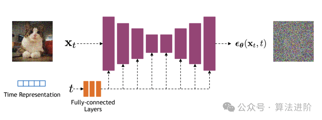
The popular Sora large model is fundamentally based on the Diffusion model, which is a deep learning-based generative model primarily used for generating continuous data like images and audio. The core idea of the Diffusion model is to transform complex data distributions into simple Gaussian distributions by gradually adding noise, and then generate data from the simple distribution by gradually removing the noise.

Algorithm Principle:

The basic idea of the Diffusion Model is to view the data generation process as a Markov chain. Starting from the target data, each step approaches random noise until reaching a pure noise state. Then, through a reverse process, the model gradually recovers to the target data from pure noise. This process is typically described by a series of conditional probability distributions.

Training Process:

1. Forward Process: Starting from real data, gradually add noise until reaching pure noise. In this process, the noise level at each step needs to be calculated and saved.

2. Reverse Process: Starting from pure noise, gradually remove noise until recovering to the target data. In this process, a neural network (usually a U-Net structure) is used to predict the noise levels at each step and generate data accordingly.

3. Optimization: Train the model by minimizing the difference between real data and generated data. Common loss functions include MSE (Mean Squared Error) and BCE (Binary Cross-Entropy).

Advantages:

1. High generation quality: Due to the gradual diffusion and recovery process, the Diffusion Model can generate high-quality data.

2. Strong interpretability: The generation process of the Diffusion Model has clear physical significance, making it easy to understand and explain.

3. Good flexibility: The Diffusion Model can handle various types of data, including images, text, and audio.

Disadvantages:

1. Long training time: Due to the multiple steps of diffusion and recovery, the training time for the Diffusion Model is relatively long.

2. High computational resource demands: To ensure generation quality, the Diffusion Model typically requires substantial computational resources, including memory and computational power.

Applicable Scenarios:

The Diffusion Model is suitable for scenarios requiring high-quality data generation, such as image generation, text generation, and audio generation. Additionally, due to its strong interpretability and good flexibility, the Diffusion Model can also be applied in other fields that require deep generative models.

Python Example Code:

import torch
import torch.nn as nn
import torch.optim as optim

# Define U-Net model
class UNet(nn.Module):
    # ... (model definition omitted)

# Define Diffusion Model
class DiffusionModel(nn.Module):
    def __init__(self, unet):
        super(DiffusionModel, self).__init__()
        self.unet = unet

    def forward(self, x_t, t):
        # x_t is the current data, t is the noise level
        # Use U-Net to predict the noise level
        noise_pred = self.unet(x_t, t)
        # Generate data based on the noise level
        x_t_minus_1 = x_t - noise_pred * torch.sqrt(1 - torch.exp(-2 * t))
        return x_t_minus_1

# Initialize model and optimizer
unet = UNet()
model = DiffusionModel(unet)
optimizer = optim.Adam(model.parameters(), lr=0.001)

# Training process
for epoch in range(num_epochs):
    for x_real in dataloader:  # Fetch real data from the data loader
        # Forward process
        x_t = x_real  # Start from real data
        for t in torch.linspace(0, 1, num_steps):
            # Add noise
            noise = torch.randn_like(x_t) * torch.sqrt(1 - torch.exp(-2 * t))
            x_t = x_t + noise * torch.sqrt(torch.exp(-2 * t))
            # Calculate predicted noise
            noise_pred = model(x_t, t)
            # Calculate loss
            loss = nn.MSELoss()(noise_pred, noise)
            # Backpropagation and optimization
            optimizer.zero_grad()
            loss.backward()
            optimizer.step()

import torch
from torch_geometric.nn import GCNConv
from torch_geometric.data import Data

# Define a simple graph structure
edge_index = torch.tensor([[0, 1, 1, 2],                           [1, 0, 2, 1]], dtype=torch.long)
x = torch.tensor([[-1], [0], [1]], dtype=torch.float)

data = Data(x=x, edge_index=edge_index)

# Define a simple two-layer graph convolutional network
class Net(torch.nn.Module):
    def __init__(self):
        super(Net, self).__init__()
        self.conv1 = GCNConv(dataset.num_features, 16)
        self.conv2 = GCNConv(16, dataset.num_classes)

    def forward(self, data):
        x, edge_index = data.x, data.edge_index
        x = self.conv1(x, edge_index)
        x = torch.relu(x)
        x = torch.dropout(x, training=self.training)
        x = self.conv2(x, edge_index)
        return torch.log_softmax(x, dim=1)

# Instantiate model, loss function, and optimizer
model = Net()
criterion = torch.nn.NLLLoss()
optimizer = torch.optim.Adam(model.parameters(), lr=0.01, weight_decay=5e-4)

# Train the model
model.train()
for epoch in range(200):
    optimizer.zero_grad()
    out = model(data)
    loss = criterion(out[data.train_mask], data.y[data.train_mask])
    loss.backward()
    optimizer.step()

# Evaluate the model on the test set
model.eval()
_, pred = model(data).max(dim=1)
correct = int((pred == data.y).sum().item())
acc = correct / int(data.y.sum().item())
print('Accuracy: {:.4f}'.format(acc))

import tensorflow as tf
import numpy as np
import random
import gym
from collections import deque

# Set hyperparameters
BUFFER_SIZE = int(1e5)  # Size of experience replay buffer
BATCH_SIZE = 64        # Number of samples to draw from replay buffer each time
GAMMA = 0.99           # Discount factor
TAU = 1e-3             # Target network update rate
LR = 1e-3              # Learning rate
UPDATE_RATE = 10       # How often to update the target network

# Define experience replay buffer class
class ReplayBuffer:
    def __init__(self, capacity):
        self.buffer = deque(maxlen=capacity)

    def push(self, state, action, reward, next_state, done):
        self.buffer.append((state, action, reward, next_state, done))

    def sample(self, batch_size):
        return random.sample(self.buffer, batch_size)

# Define DQN model class
class DQN:
    def __init__(self, state_size, action_size):
        self.state_size = state_size
        self.action_size = action_size
        self.model = self._build_model()

    def _build_model(self):
        model = tf.keras.Sequential()
        model.add(tf.keras.layers.Dense(24, input_dim=self.state_size, activation='relu'))
        model.add(tf.keras.layers.Dense(24, activation='relu'))
        model.add(tf.keras.layers.Dense(self.action_size, activation='linear'))
        model.compile(loss='mse', optimizer=tf.keras.optimizers.Adam(lr=LR))
        return model

    def remember(self, state, action, reward, next_state, done):
        self.replay_buffer.push((state, action, reward, next_state, done))

    def act(self, state):
        if np.random.rand() <= 0.01:
            return random.randrange(self.action_size)
        act_values = self.model.predict(state)
        return np.argmax(act_values[0])

    def replay(self, batch_size):
        minibatch = self.replay_buffer.sample(batch_size)
        for state, action, reward, next_state, done in minibatch:
            target = self.model.predict(state)
            if done:
                target[0][action] = reward
            else:
                Q_future = max(self.target_model.predict(next_state)[0])
                target[0][action] = reward + GAMMA * Q_future
            self.model.fit(state, target, epochs=1, verbose=0)
        if self.step % UPDATE_RATE == 0:
            self.target_model.set_weights(self.model.get_weights())

    def load(self, name):
        self.model.load_weights(name)

    def save(self, name):
        self.model.save_weights(name)

# Create environment
env = gym.make('CartPole-v1')
state_size = env.observation_space.shape[0]
action_size = env.action_space.n

# Initialize DQN and replay buffer
dqn = DQN(state_size, action_size)
replay_buffer = ReplayBuffer(BUFFER_SIZE)

# Training process
total_steps = 10000
for step in range(total_steps):
    state = env.reset()
    state = np.reshape(state, [1, state_size])
    for episode in range(100):
        action = dqn.act(state)
        next_state, reward, done, _ = env.step(action)
        next_state = np.reshape(next_state, [1, state_size])
        replay_buffer.remember(state, action, reward, next_state, done)
        state = next_state
        if done:
            break
    if replay_buffer.buffer.__len__() > BATCH_SIZE:
        dqn.replay(BATCH_SIZE)

Edited by: Wang Jing