Introduction

To achieve this machine learning model, we will launch Generative Adversarial Networks (GANs) and input data containing features of “The Simpsons” images. By the end of this article, you will be familiar with the basics behind GANs, and you can also build your own generative model.

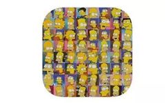
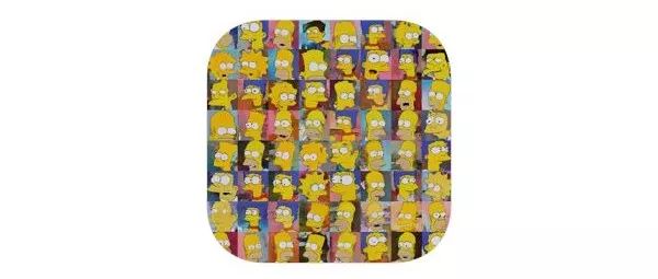
To better understand the functionality of GANs, take a look at the changes during the training process of The Simpsons below.

Isn’t it amazing?

Let’s explore some theory to better understand how it actually works.

Let’s start our journey with GANs by defining the problem we want to solve.

We provide a set of images as input, and based on that input, samples will be generated as output.

Input Images -> GAN -> Output Samples

According to the definition of the problem above, GANs belong to unsupervised learning because we do not input any expert knowledge (such as sample labeling in classification tasks) into the model.

Generating samples based on a given dataset without any human supervision sounds very promising.

Let’s understand how GANs make this possible!

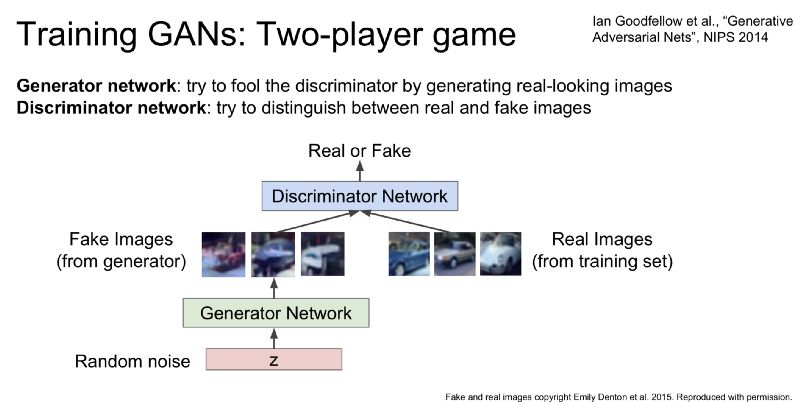
The underlying principle behind GANs is that it involves two adversarial neural networks, namely the generator and the discriminator, within a zero-sum game framework.

Generator

The generator takes random noise as input and generates samples as output. Its goal is to produce samples that look fake but are convincing enough for the discriminator to believe they are real images. We can think of the generator as a forger.

Discriminator

The discriminator receives real images from the input dataset and fake images from the generator and determines whether the image is real or fake. We can think of the discriminator as a police officer catching a bad guy and letting the good guy go.

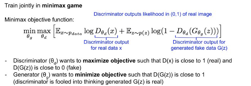
Minimax Representation

If we think again about the goals of the discriminator and generator, we can see they are oppositional. If the discriminator succeeds in distinguishing, then the generator fails in generating, and vice versa. This is why we represent the GANs framework as a minimax game framework rather than an optimization problem.

http://cs231n.stanford.edu/slides/2017/cs231n_2017_lecture13.pdf

http://cs231n.stanford.edu/slides/2017/cs231n_2017_lecture13.pdf

GANs are designed to reach a Nash equilibrium, in which each player cannot reduce their cost without changing the other player’s situation.

For those familiar with game theory and minimax algorithms, this idea seems easy to understand. For those who are not familiar, it is recommended to look at articles that explain the basics of minimax algorithms.

Data Flow and Backpropagation

Although the minimax representation of two adversarial networks seems reasonable, we still do not know how to enable them to self-improve, ultimately transforming random noise into a realistic image.

Random Noise to Realistic Images

Let’s start with the discriminator.

The discriminator receives real images and fake images and tries to determine their authenticity. As the designers of the system, we know whether they are from the real dataset or generated by the generator. Therefore, we can use this information to label them accordingly and perform a classification backpropagation to allow the discriminator to learn repeatedly, improving its ability to distinguish between real and fake images. If the discriminator correctly classifies the fake images as fake and the real images as real, we provide positive feedback in the form of loss gradients. If it fails to classify correctly, it receives negative feedback. This mechanism helps the discriminator learn better.

Now let’s move to the generator.

The generator takes random noise as input and outputs samples to deceive the discriminator into thinking they are real images. Once the output from the generator passes through the discriminator, we can know whether the discriminator has judged it to be a real image or a fake image. We can relay this information back to the generator for another backpropagation. If the discriminator judges the generator’s output as real, it means the generator is performing well and should be rewarded. On the other hand, if the discriminator identifies it as fake, the generator has failed and receives negative feedback as punishment.

If you think about it carefully, you will find that through the above method, we have combined game theory, supervised learning, and a bit of reinforcement learning to solve the unsupervised learning problem.

The data flow of GANs can be represented in the following flowchart.

https://www.oreilly.com/ideas/deep-convolutional-generative-adversarial-networks-with-tensorflow

And some basic mathematics.

https://medium.com/@jonathan_hui/gan-whats-generative-adversarial-networks-and-its-application-f39ed278ef09

I hope you are not intimidated by the formulas above; they will become very easy to understand as we begin the actual implementation of GAN.

As always, you can find the complete code repository for the image generator on GitHub. Everything is in a single Jupyter notebook file, which you can run on any platform you want to use. More information about the dataset can be found in this file, and you can follow it accordingly.

Since we need to handle image data, we have to find a more efficient way to represent it. This can be achieved by DCGAN, which stands for Deep Convolutional Generative Adversarial Networks.

Model

In our project, we use a well-tested model structure proposed by Radford et al. in 2015, as shown in the figure below.

You can find our implementation of this model in TensorFlow in the discriminator and generator functions here.

As you can see in the visualization above, the generator and discriminator have almost the same structure but are inverted. We won’t delve into the details of CNNs now, but if you are more concerned about the underlying details, you can check out the following article:

https://towardsdatascience.com/image-classifier-cats-vs-dogs-with-convolutional-neural-networks-cnns-and-google-colabs-4e9af21ae7a8

Loss Function

To allow our discriminator and generator to learn multiple times, we need to provide a loss function to enable backpropagation.

def model_loss(input_real, input_z, output_channel_dim:
  g_model = generator(input_z, output_channel_dim, True)

  noisy_input_real = input_real + tf.random_normal(shape=tf.shape(input_real),
                           mean=0.0,
                           stddev=random.uniform(0.0, 0.1),
                           dtype=tf.float32)

  d_model_real, d_logits_real = discriminator(noisy_input_real, reuse=False)
  d_model_fake, d_logits_fake = discriminator(g_model, reuse=True)

  d_loss_real = tf.reduce_mean(tf.nn.sigmoid_cross_entropy_with_logits(logits=d_logits_real,
                                     labels=tf.ones_like(d_model_real)*random.uniform(0.9, 1.0)))
  d_loss_fake = tf.reduce_mean(tf.nn.sigmoid_cross_entropy_with_logits(logits=d_logits_fake,
                                     labels=tf.zeros_like(d_model_fake)))
  d_loss = tf.reduce_mean(0.5 * (d_loss_real + d_loss_fake))
  g_loss = tf.reduce_mean(tf.nn.sigmoid_cross_entropy_with_logits(logits=d_logits_fake,
                                  labels=tf.ones_like(d_model_fake)))
  return d_loss, g_loss

Although the loss declaration above is consistent with the theoretical explanation in the previous chapter, you may notice two things:

• Gaussian noise is added to the input of real images in line four.

• In line twelve, one-sided label smoothing is applied to the real images identified by the discriminator.

You will find that training GANs is quite challenging because there are two loss functions (one for the generator and one for the discriminator), and finding a balance between them is key to achieving good results.

Since it is common for the discriminator to be larger than the generator in practice, sometimes we need to reduce the discriminator, and we are achieving that through the modifications above. We will introduce other techniques for achieving balance later.

Optimization

We use the following Adam optimization algorithm to optimize our model.

def model_optimizers(d_loss, g_loss):
  t_vars = tf.trainable_variables()
  g_vars = [var for var in t_vars if var.name.startswith("generator")]
  d_vars = [var for var in t_vars if var.name.startswith("discriminator")]

  update_ops = tf.get_collection(tf.GraphKeys.UPDATE_OPS)
  gen_updates = [op for op in update_ops if op.name.startswith('generator')]

  with tf.control_dependencies(gen_updates):
     d_train_opt = tf.train.AdamOptimizer(learning_rate=LR_D, beta1=BETA1).minimize(d_loss, var_list=d_vars)
    g_train_opt = tf.train.AdamOptimizer(learning_rate=LR_G, beta1=BETA1).minimize(g_loss, var_list=g_vars)
  return d_train_opt, g_train_opt

Similar to the declaration of the loss function, we can also use appropriate learning rates to balance the discriminator and generator.

LR_D = 0.00004
LR_G = 0.0004
BETA1 = 0.5

Since the hyperparameters above are use-case specific, feel free to adjust them. But also remember that GANs are very sensitive to changes in learning rates, so please fine-tune them very carefully.

Training

Finally, we can start training.

def train(get_batches, data_shape, checkpoint_to_load=None):
  input_images, input_z, lr_G, lr_D = model_inputs(data_shape[1:], NOISE_SIZE)
  d_loss, g_loss = model_loss(input_images, input_z, data_shape[3])
  d_opt, g_opt = model_optimizers(d_loss, g_loss)

  with tf.Session() as sess:
    sess.run(tf.global_variables_initializer())
    epoch = 0
    iteration = 0
    d_losses = []
    g_losses = []

    for epoch in range(EPOCHS): 
      epoch += 1
      start_time = time.time()

      for batch_images in get_batches:
         iteration += 1
        batch_z = np.random.uniform(-1, 1, size=(BATCH_SIZE, NOISE_SIZE))
        _ = sess.run(d_opt, feed_dict={input_images: batch_images, input_z: batch_z, lr_D: LR_D})
        _ = sess.run(g_opt, feed_dict={input_images: batch_images, input_z: batch_z, lr_G: LR_G})
        d_losses.append(d_loss.eval({input_z: batch_z, input_images: batch_images}))
        g_losses.append(g_loss.eval({input_z: batch_z}))

       summarize_epoch(epoch, time.time()-start_time, sess, d_losses, g_losses, input_z, data_shape)

The above function contains a standard machine learning training scheme. It divides our dataset into batches of a specific size and begins training for a given number of iterations.

The core training part is in lines 22 to 23, where the discriminator and generator are trained. Similar to the loss function and learning rates, this is also a place where the balance between the discriminator and generator can be achieved. Some researchers have found that adjusting the training run ratio between the discriminator and generator is beneficial for results. In my project, a 1:1 ratio performed the best, but you can use it freely.

Additionally, I also used the following hyperparameters, but they are not set in stone, and you can boldly modify them.

IMAGE_SIZE = 128
NOISE_SIZE = 100
BATCH_SIZE = 64
EPOCHS = 300

It is very important to frequently monitor the model’s loss function and its performance. I recommend observing after every batch, as shown in the code snippet above. Let’s take a look at some samples generated during the training process.

We can clearly see that our model is improving and learning to generate more realistic Simpsons.

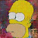
Let’s focus on the main character, the head of the household, Homer Simpson (some also call him Homer).

Random noise at batch 0

Yellow at batch 5

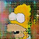
Head shape at batch 15

Brown beard at batch 50

Mouth at batch 100

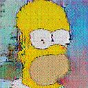
Eyeballs at batch 200

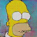
Head shape at batch 250

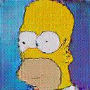
Homer smiling slightly at batch 300

Homer Simpson evolving over time

Final Results

Ultimately, after 8 hours of training over 300 batches on an NVIDIA P100 (Google Cloud), we can see that our artificially generated Simpsons family truly begins to look real! Take a look at some of the better samples selected below.

As expected, there are also some interestingly abnormal faces.

Although GAN image generation has proven to be very successful, this is not the only possible application of Generative Adversarial Networks. For example, take a look at the image-to-image transformation implemented using CycleGAN below.

(Source: https://junyanz.github.io/CycleGAN/)

Isn’t it amazing?

I suggest you delve deeper into the field of GANs, as there is still much to explore!

Don’t forget to check out this project on GitHub:

https://github.com/gsurma/image_generator

Editor: Liu Yangke

This article is reprinted with permission from the public account: AI Research Society

Recommended Learning

(This series of courses consists of 9 single classes, divided into 18 micro-classes)

Learning address:

https://campus.swarma.org/gpac=412

Or clickRead the original textto view

Recommended Reading

Follow the AI Learning Society public account