Author: Zhong Yangyang
Reviewed by: Chen Zhiyan





This article is approximately 2500 words long and is recommended to be read in 5 minutes.
This article provides a brief introduction to the basic concepts of Graph Neural Networks and typical models.

A graph (Graph) is a type of data structure that can naturally model the complex relationships among a set of entities in real-world scenarios. In reality, many data often appear in the form of graphs, such as social networks, e-commerce shopping, and protein interaction relationships. Therefore, in recent years, research on using intelligent methods to model and analyze graph structures has received increasing attention, among which Graph Neural Networks (GNNs), based on deep learning, have been widely applied in various fields such as social sciences and natural sciences due to their outstanding performance.

Basic Concepts

1.1 Basic Concepts of Graphs

Graphs are typically represented as G=(V, E), where V represents the set of nodes and E represents the set of edges. For two adjacent nodes u and v, the edge between these two nodes is denoted as e=(u,v). The edge between two nodes can be directed or undirected. If directed, it is called a Directed Graph; otherwise, it is called an Undirected Graph.

1.2 Graph Representation

In Graph Neural Networks, common representation methods include adjacency matrix, degree matrix, and Laplacian matrix.

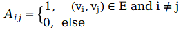
1) Adjacency Matrix

It is used to represent the relationships between nodes in a graph. For a simple graph with n nodes, the adjacency matrix is::

2) Degree Matrix

The degree (Degree) of a node indicates the number of edges connected to that node, denoted as d(v). For a simple graph G=(V, E) with n nodes, its degree matrix D is, which is also a diagonal matrix.

3) Laplacian Matrix

For a simple graph G=(V, E) with n nodes, its Laplacian matrix is defined as L=D-A, where D and A are the degree matrix and adjacency matrix mentioned above. After normalization, we have.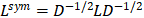

1.3 Basic Concepts of Graph Neural Networks

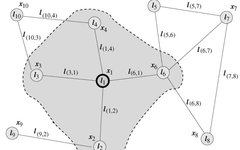
Graph Neural Networks (GNN) were first proposed by Marco Gori [1], Franco Scarselli [2,3], and others, who extended neural network methods to the field of graph data computation. In Scarselli’s paper, a typical graph is shown in Figure 1:

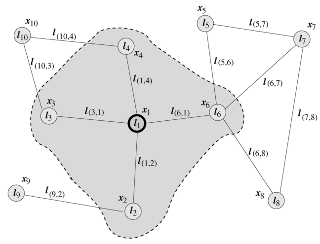
Figure 1 Typical Graph Neural Network

To update the node state based on the input node neighbor information, the local transfer function f is defined in the form of a recursive function, where each node updates its representation h based on the surrounding neighbor nodes and the edges connected to them. To obtain the node output o, a local output function g is introduced. Therefore, we have the following definitions:

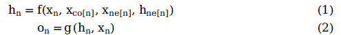
where x represents the node input, h represents the node hidden state, ne[n] represents the set of neighbor nodes of node n, and co[n] represents the set of edges adjacent to node n. Taking node L1 in Figure 1 as an example, X1 is its input feature,contains node 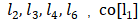, and contains edge.

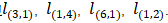Stacking all local transfer functions f, we have:

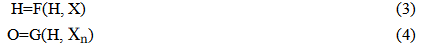
where F is the Global Transition Function and G is the Global Output Function.

According to the Banach fixed-point theorem [4], assuming that F in formula (3) is a contraction mapping, then the fixed point H can be uniquely determined and can be iteratively solved as follows:

Based on the fixed-point theorem, for any initial value, GNN will converge to the solution described by formula (3) according to formula (5).

Classic Models

2.1 GCN – The Pioneer

In 2017, Thomas N. Kipf and others proposed GCN [5]. Its structure is shown in Figure 2:

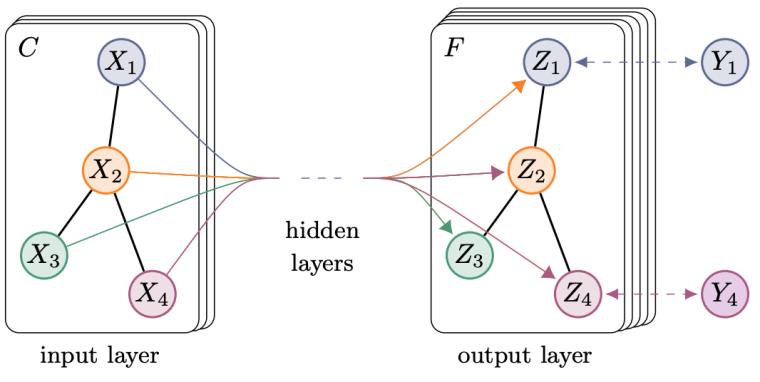
Figure 2 GCN proposed by Thomas N. Kipf et al.

Assuming we need to construct a two-layer GCN with activation functions ReLU and Softmax, the overall forward propagation formula is as follows:

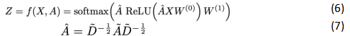
where W0 represents the weight matrix of the first layer, W1 represents the weight matrix of the second layer, and X is the node feature,is equal to the adjacency matrix A plus the identity matrix,isthe degree matrix.

From the above forward propagation formula and diagram, GCN seems to have no difference from the basic GNN. Next, we provide the transmission formula of GCN (8):

Observe the product of the normalized matrix and the feature vector matrix:

Source:https://www.zhihu.com/question/426784258

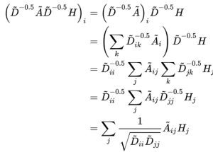
It can be observed that GCN introduces the degree matrix D for normalizing the adjacency matrix, and the inter-layer propagation will no longer simply average the features of neighboring nodes. It not only considers the degree of node i but also the degree of adjacent node j, so for nodes with a higher degree, their contribution during aggregation will be less.

Article [5] has experimentally demonstrated the outstanding performance of GCN. Even without training, the features extracted are already very good. The author conducted an experiment using club relationship network data, as shown in Figure 3:

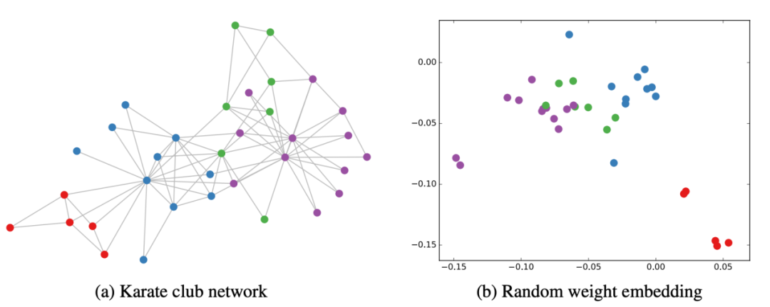
Figure 3 GCN Automatically Clustering Spatially From the above figure, it can be observed that using randomly initialized GCN for feature extraction, the embeddings extracted by GCN have already clustered spatially.

2.2 GAT – Attention Mechanism

GAT [6] is a typical graph neural network based on the attention mechanism. The structure of the Graph Attention Network is shown in Figure 4, where the features of nodes i and j are used as output to calculate the attention weights between the two nodes.

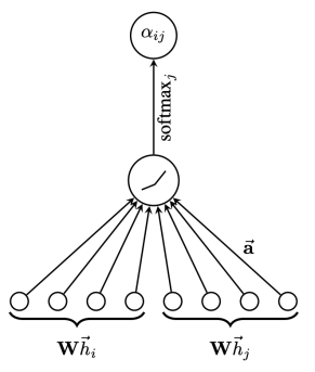
Figure 4 Graph Attention Network Structure

The calculation method of the attention coefficients (Attention Coefficients) for nodes i and j is:

where W is a linear mapping with shared parameters for increasing the dimensionality of node features, h is the node’s features, and a(W, W) can represent the similarity calculated by the inner product of two vectors. After applying softmax, we obtain the attention weights:

Thus, the attention weight calculation formula is as follows:

where Ni represents the neighboring nodes of node i, and || denotes feature concatenation.

The final output of the node is as shown in the following formula, which is easy to understand: it assigns different weights to neighboring nodes to aggregate information.

In article [6], the author also introduced multi-head attention, with the structure shown in Figure 5 and the formula as (13):

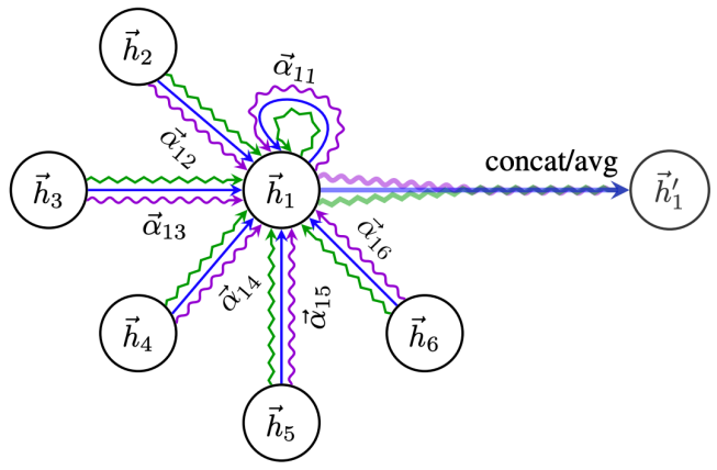
Figure 5 Multi-Head Attention Mechanism Structure

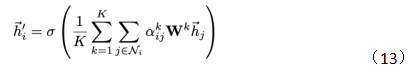
Multi-head attention essentially introduces several independent attention mechanisms in parallel, which can extract multiple meanings from the information and prevent overfitting.

2.3 GraphSAGE – Inductive Learning Framework

When mentioning the GraphSAGE [7] model, we must also mention GCN. Let’s review the iterative formula of GCN:

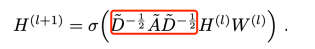
The operation performed at the red frame position in the figure can be simply understood as a normalization transformation of the adjacency matrix A. Removing this part shows that the remaining structure is equivalent to a deep neural network. By adding the red part, the matrix multiplication essentially sums the features of nodes and their neighboring nodes.

GraphSAGE differs from GCN in that while GCN simply adds features, GraphSAGE supports aggregation methods such as max-pooling, LSTM, and mean. Additionally, the biggest difference between GraphSAGE and GCN is that GCN is a transductive method, meaning it requires all nodes to be present in the graph and cannot handle new nodes. In contrast, GraphSAGE is inductive, allowing it to generate embeddings for unseen nodes.

The propagation method of GraphSAGE is shown in Figure 6:

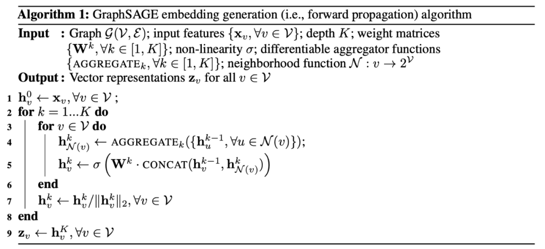
Figure 6 Propagation Method of GraphSAGE

It can be seen that for a certain node v in graph G, if we need to aggregate k layers of information, we first have a for loop for the number of layers, and the second loop is to traverse the neighboring nodes of node v. Then, through the aggregation function AGGEGATE (which can be mean, max, LSTM, or others), we aggregate the information from k-1 layers of neighboring nodes, obtaining the aggregated k-layer neighboring node information, which is then concatenated with the k-1 layer information of node v, and calculated using weight parameters W to obtain k-layer information about node v.

To be more intuitive, let’s look at the following figure:

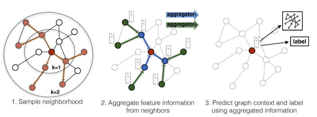
Figure 7 Node Propagation Method in Graph

In the above, the red node is the target node. In one step, we randomly sample the first-order and second-order neighbors of the red node. Then, using the aggregation strategy, we aggregate the feature information from the second-order neighbors to the target node, and the updated representation of the target node can be applied to different task needs.

Conclusion

In summary, compared to GCN, GraphSAGE can avoid the need to load the entire network at once, can flexibly design aggregation methods, and has transductive properties. It can adapt to changes in the test set nodes without needing to retrain the model due to changes in the Laplacian matrix as GCN does.

References[1] M. Gori, G. Monfardini and F. Scarselli, “A new model for learning in graph domains,” Proceedings. 2005 IEEE International Joint Conference on Neural Networks, 2005., 2005, pp. 729-734 vol. 2, doi: 10.1109/IJCNN.2005.1555942.[2] Scarselli F , Tsoi A C , Gori M , et al. Graphical-Based Learning Environments for Pattern Recognition[J]. DBLP, 2004.[3] Franco, Scarselli, Marco, Gori, Ah Chung, Tsoi, Markus, Hagenbuchner, Gabriele, Monfardini. The graph neural network model.[J]. IEEE transactions on neural networks, 2009, 20(1):61-80. DOI:10.1109/TNN.2008.2005605.[4] MA Khamsi, WA Kirk. An Introduction to Metric Spaces and Fixed Point Theory. 2011.[5] Kipf T N , Welling M . Semi-Supervised Classification with Graph Convolutional Networks[J]. 2016.[6] Velikovi P , Cucurull G , Casanova A , et al. Graph Attention Networks[J]. 2017.[7] W. Hamilton, Z. Ying and J. Leskovec, “Inductive representation learning on large graphs” in Advances in Neural Information Processing Systems, pp. 1025-1035, 2017.

Author Biography

Zhong Yangyang, Volunteer at Datapi Research Department, graduated with a master’s degree from Northeastern University, mainly researching computer vision, graph neural networks, etc.

Editor: Yu Tengkai

Proofreader: Lin Yilin

Introduction to Datapi Research Department

The Datapi Research Department was established in early 2017, dividing into multiple groups based on interests, each group follows the overall knowledge sharing and practical project planning of the research department while having its own characteristics:

Algorithm Model Group: Actively participates in competitions like Kaggle and publishes original hands-on teaching series articles;

Research Analysis Group: Investigates the application of big data through interviews and explores the beauty of data products;

System Platform Group: Tracks the cutting edge of big data & AI system platform technology and engages with experts;

Natural Language Processing Group: Focuses on practice, actively participates in competitions, and plans various text analysis projects;

Manufacturing Big Data Group: Upholds the dream of an industrial power, combines industry, academia, research, and government to explore data value;

Data Visualization Group: Merges information with art, explores the beauty of data, and learns to tell stories using visualization;

Web Crawler Group: Crawls web information and collaborates with other groups to develop creative projects.

Click on the end of the article “Read Original” to sign up for Datapi Research Department Volunteers, there is always a group that suits you~

Reprint Notice

If you need to reprint, please indicate the author and source prominently at the beginning of the article (Transcribed from: Datapi THU ID: DatapiTHU), and place a prominent QR code at the end of the article. For articles with original identifiers, please send the 【Article Name – Pending Authorized Public Account Name and ID】 to the contact email to apply for whitelist authorization and edit according to requirements.

Unauthorized reprints and adaptations will be legally pursued.

Click “Read Original” to join the organization~