

Source: Read Chip Technology
This article is approximately 8000 words, and it is recommended to read in 16 minutes.
Step-by-step guide on how to use Convolutional Neural Networks to build an image classifier.

Image source: pexels.com
Neural networks consist of neurons with weights and biases. By adjusting these weights and biases during training, a good learning model can be proposed. Each neuron receives a set of inputs, processes them in some way, and then outputs a value. If a neural network is constructed with multiple layers, it is called a deep neural network. The branch of artificial intelligence that deals with these deep neural networks is called deep learning.
One of the main drawbacks of ordinary neural networks is that they ignore the structure of input data. Before feeding the data into the neural network, all data is converted into one-dimensional arrays. This works for regular data but encounters difficulties when processing images.
Considering that grayscale images have a 2D structure, the spatial arrangement of pixels contains a lot of hidden information. Ignoring this information means losing many potential patterns. This is why Convolutional Neural Networks (CNNs) were introduced for image processing. CNNs take into account the 2D structure of images when processing them.
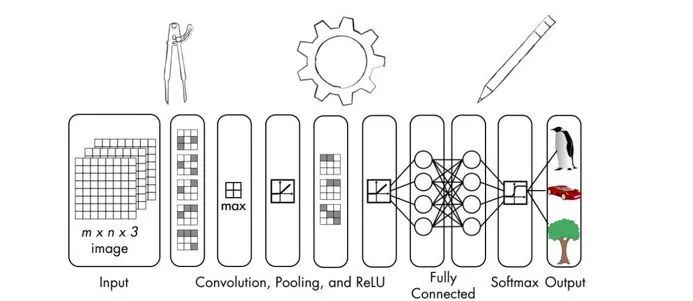
CNNs are also composed of neurons with weights and biases. These neurons receive input data, process it, and then output information. The goal of the neural network is to transfer the raw image data from the input layer to the correct class in the output layer. The difference between ordinary neural networks and CNNs lies in the types of layers used and how the input data is processed. Assuming the input to the CNN is an image, this allows it to extract image-specific attributes. This makes CNNs more efficient in handling images. So, how is a CNN constructed?
Architecture of CNN
When using ordinary neural networks, input data needs to be converted into a single vector. This vector serves as the input to the neural network and then passes through the various layers of the neural network. In these layers, each neuron is connected to all neurons in the previous layer. It is worth noting that neurons in the same layer do not connect to each other; they only connect to neurons in adjacent layers. The last layer in the network is the output layer, which represents the final output.
If this structure is used for image processing, it quickly becomes hard to manage. For example, an image dataset made up of 256×256 RGB images would have 256 * 256 * 3 = 196,608 weights. Please note that this is only for a single neuron! Each layer has multiple neurons, so the number of weights increases rapidly. This means that during training, the model will require a large number of parameters to adjust the weights. This is why this structure is complex and time-consuming. Connecting each neuron to every neuron in the previous layer is called fully connected, which is clearly not suitable for image processing.
CNNs explicitly consider the structure of images when processing data. Neurons in a CNN are arranged in three dimensions—width, height, and depth. Each neuron in the current layer is connected to a small patch of the previous layer’s output. It is like overlaying an NxN filter on the input image. This is in contrast to fully connected layers, where each neuron in a fully connected layer is connected to all neurons in the previous layer.
Since a single filter cannot capture all the nuances of an image, it takes multiple times (let’s say M times) to ensure that all details are captured. These M filters act as feature extractors. If you look at the outputs of these filters, you can see features extracted by the layers, such as edges, corners, etc. This applies to the initial layers in a CNN. As image processing progresses through the layers of the neural network, later layers will extract higher-level features.
Types of Layers in CNN
Having understood the architecture of CNN, let’s continue to look at the types of layers used to build CNNs. CNNs typically use the following types of layers:
-
Input Layer: Used for inputting raw image data.
-
Convolutional Layer: This layer computes the convolution between the neurons and various slices in the input.
Quick overview of image convolution portal:
http://web.pdx.edu/~jduh/courses/Archive/geog481w07/Students/Ludwig_ImageConvolution.pdf.
The convolutional layer essentially computes the dot product between the weights and slices of the output from the previous layer.
-
Activation Layer: This layer applies an activation function to the output of the previous layer. This function is similar to max(0, x). This layer needs to add a nonlinear mapping to the neural network so that it can generalize well to any type of function.
-
Pooling Layer: This layer samples the output from the previous layer, generating a structure with smaller dimensions. When processing images in the network, pooling helps retain only the prominent parts. Max pooling is the most commonly used pooling layer, which selects the maximum value within a given KxK window.
-
Fully Connected Layer: This layer computes the output from the last layer. The output size is 1x1xL, where L is the number of classes in the training dataset.
From the input layer of the neural network to the output layer, the input image will be transformed from pixel values to final class scores. Many different CNN architectures have been proposed, and this is an active research area. The accuracy and robustness of the model depend on many factors—the types of layers, the depth of the network, the arrangement of various types of layers in the network, the functions chosen for each layer, and the training data, etc.
Building a Linear Regression Model Based on Perceptron
Next, we will discuss how to build a linear regression model using a perceptron.
This section will use TensorFlow. It is a popular deep learning package widely used to build various real-world systems. In this section, we will familiarize ourselves with how it works. First, install the package before using it.
Installation instructions portal:
https://www.tensorflow.org/get_started/os_setup.
Once it is installed, create a new Python program and import the following packages:
import numpy as np
import matplotlib.pyplot as plt
import tensorflow as tf
Fit the model to the generated data points. Define the number of points to generate:
# Define the number of points to generate
num_points = 1200
Define the parameters that will be used to generate the data. Using a linear model: y = mx + c:
# Generate the data based on equation y = mx + c
data = []
m = 0.2
c = 0.5
for i in range(num_points):
# Generate ‘x’
x = np.random.normal(0.0, 0.8)
Generated noise causes data to change:
# Generate some noise
noise = np.random.normal(0.0, 0.04)
Calculate the value of y using the following equation:
# Compute ‘y’
y = m*x + c + noise
data.append([x, y])
After completing the iteration, separate the data into input and output variables:
# Separate x and y
x_data = [d[0] for d in data]
y_data = [d[1] for d in data
Plot the data:
# Plot the generated data
plt.plot(x_data, y_data, ‘ro’)
plt.title(‘Input data’)
plt.show()
Generate weights and biases for the perceptron. Weights are generated by a uniform random number generator, and biases are set to zero:
# Generate weights and biases
W = tf.Variable(tf.random_uniform([1], -1.0, 1.0))
b = tf.Variable(tf.zeros([1]))
Define the equation using TensorFlow variables:
# Define equation for ‘y’
y = W * x_data + b
Define the loss function used in the training process. The optimizer will minimize the value of the loss function as much as possible.
# Define how to compute the loss
loss = tf.reduce_mean(tf.square(y – y_data))
Define the gradient descent optimizer and specify the loss function:
# Define the gradient descent optimizer
optimizer = tf.train.GradientDescentOptimizer(0.5)
train = optimizer.minimize(loss)
All variables are in place, but not initialized yet. Next:
# Initialize all the variables
init = tf.initialize_all_variables()
Start the TensorFlow session and run it with the initializer:
# Start the tensorflow session and run it
sess = tf.Session()
sess.run(init)
Start training:
# Start iterating
num_iterations = 10
for step in range(num_iterations):
# Run the session
sess.run(train)
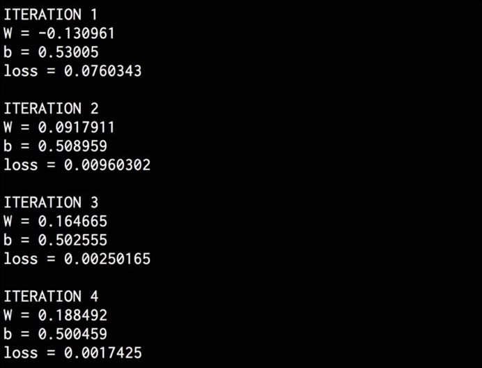
Print the training progress. During iterations, the loss parameter will continue to decrease:
# Print the progress
print(‘\nITERATION’, step+1)
print(‘W =’, sess.run(W)[0])
print(‘b =’, sess.run(b)[0])
print(‘loss =’, sess.run(loss))
Plot the generated data and overlay the predicted model on top. In this case, the model is a line:
# Plot the input data
plt.plot(x_data, y_data, ‘ro’)
# Plot the predicted output line
plt.plot(x_data, sess.run(W) * x_data + sess.run(b))
Set the parameters for plotting:
# Set plotting parameters
plt.xlabel(‘Dimension 0’)
plt.ylabel(‘Dimension 1’)
plt.title(‘Iteration ‘ + str(step+1) + ‘ of ‘ + str(num_iterations))
plt.show()
The complete code is given in the linear_regression.py file. Running the code will show the following screenshot displaying the input data:

If you close this window, you will see the training process. The first iteration looks like this:
As you can see, the line is completely off the model. Close this window to go to the next iteration:
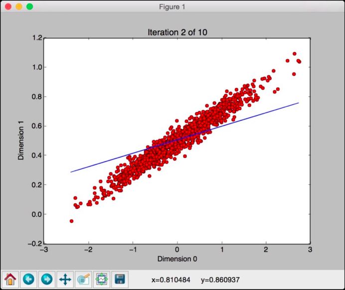
This line seems better, but it is still off the model. Close this window and continue iterating:
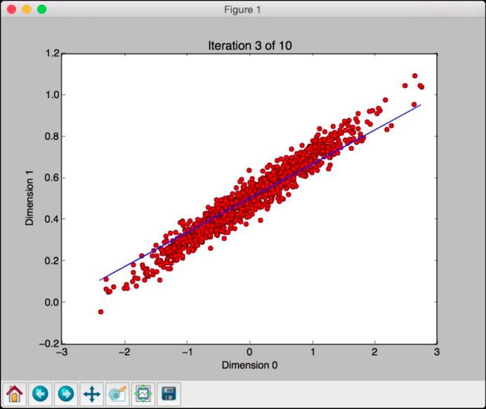
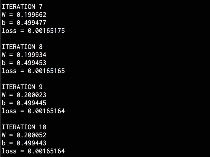
It looks like this line is getting closer to the true model. If you continue to iterate like this, the model will improve. The eighth iteration looks like this:
The line fits the data very well. You will see the following on the terminal:
After completing the training, you will see the following on the terminal:
Building an Image Classifier Using a Single-Layer Neural Network
How to create a single-layer neural network using TensorFlow and use it to build an image classifier? Use the MNIST image dataset to build the system. It is a dataset containing images of handwritten digits. The goal is to build a classifier that can correctly identify the digits in each image.
Image source: pexels.com
Create a new Python program and import the following packages:
import argparse
import tensorflow as tf
from tensorflow.examples.tutorials.mnist import input_data
Define a function to parse input parameters:
def build_arg_parser():
parser = argparse.ArgumentParser(description=’Build a classifier using
\MNIST data’)
parser.add_argument(‘–input-dir’, dest=’input_dir’, type=str,
default=’./mnist_data’, help=’Directory for storing data’)
return parser
Define the main function and parse input parameters:
if __name__ == ‘__main__’:
args = build_arg_parser().parse_args()
Extract MNIST image data. The one_hot flag specifies that one-hot encoding will be used in the labels. This means if there are n classes, the label for a given data point will be an array of length n. Each element in this array corresponds to a specific class. To specify a class, the value at the corresponding index will be set to 1, and all other values will be 0:
# Get the MNIST data
mnist = input_data.read_data_sets(args.input_dir, one_hot=True)
The images in the database are 28 x 28 pixels. They need to be converted to a one-dimensional array to create the input layer:
# The images are 28×28, so create the input layer
# with 784 neurons (28×28=784)
x = tf.placeholder(tf.float32, [None, 784])
Create a single-layer neural network with weights and biases. There are 10 distinct digits in the database. The number of neurons in the input layer is 784, and the number of neurons in the output layer is 10:
# Create a layer with weights and biases. There are 10 distinct
# digits, so the output layer should have 10 classes
W = tf.Variable(tf.zeros([784, 10]))
b = tf.Variable(tf.zeros([10]))
Create the equation for training:
# Create the equation for ‘y’ using y = W*x + b
y = tf.matmul(x, W) + b
Define the loss function and gradient descent optimizer:
# Define the entropy loss and the gradient descent optimizer
y_loss = tf.placeholder(tf.float32, [None, 10])
loss = tf.reduce_mean(tf.nn.softmax_cross_entropy_with_logits(y, y_loss))
optimizer = tf.train.GradientDescentOptimizer(0.5).minimize(loss)
Initialize all variables:
# Initialize all the variables
init = tf.initialize_all_variables()
Create a TensorFlow session and run:
# Create a session
session = tf.Session()
session.run(init)
Start the training process. Use the current batch to run the optimizer for training, then continue to the next batch for the next iteration. The first step of each iteration is to get the next batch of images:
# Start training
num_iterations = 1200
batch_size = 90
for _ in range(num_iterations):
# Get the next batch of images
x_batch, y_batch = mnist.train.next_batch(batch_size)
Run the optimizer on this batch of images:
# Train on this batch of images
session.run(optimizer, feed_dict = {x: x_batch, y_loss: y_batch})
After the training process ends, compute the accuracy using the test dataset:
# Compute the accuracy using test data
predicted = tf.equal(tf.argmax(y, 1), tf.argmax(y_loss, 1))
accuracy = tf.reduce_mean(tf.cast(predicted, tf.float32))
print(‘\nAccuracy =’, session.run(accuracy, feed_dict = {
x: mnist.test.images,
y_loss: mnist.test.labels}))
The complete code is given in the single_layer.py file. Running the code will download the data into a folder named mnist_data in the current directory. This is the default option. If you want to change it, you can do so using input parameters. After running the code, you will see the following output on the terminal:
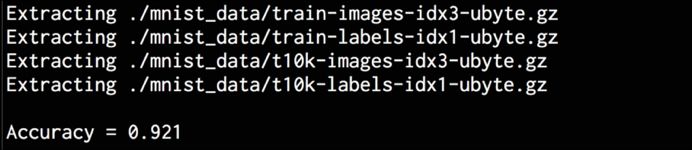
As shown in the terminal printout, the model’s accuracy is 92.1%.
Building an Image Classifier Using Convolutional Neural Networks
The image classifier from the previous section performed poorly. Achieving 92.1% on the MNIST dataset is relatively easy. How can we achieve higher accuracy by using Convolutional Neural Networks (CNNs)? Below we will build an image classifier using the same dataset but with CNN instead of a single-layer neural network.
Create a new Python program and import the following packages:
import argparse
import tensorflow as tf
from tensorflow.examples.tutorials.mnist import input_data
Define a function to parse input parameters:
def build_arg_parser():
parser = argparse.ArgumentParser(description=’Build a CNN classifier \
using MNIST data’)
parser.add_argument(‘–input-dir’, dest=’input_dir’, type=str,
default=’./mnist_data’, help=’Directory for storing data’)
return parser
Define a function to create values for weights in each layer:
def get_weights(shape):
data = tf.truncated_normal(shape, stddev=0.1)
return tf.Variable(data)
Define a function to create values for biases in each layer:
def get_biases(shape):
data = tf.constant(0.1, shape=shape)
return tf.Variable(data)
Define a function to create layers based on input shape:
def create_layer(shape):
# Get the weights and biases
W = get_weights(shape)
b = get_biases([shape[-1]])
return W, b
Define a function to perform 2D convolution:
def convolution_2d(x, W):
return tf.nn.conv2d(x, W, strides=[1, 1, 1, 1],
padding=’SAME’)
Define a function to perform 2×2 max pooling:
def max_pooling(x):
return tf.nn.max_pool(x, ksize=[1, 2, 2, 1],
strides=[1, 2, 2, 1], padding=’SAME’)
Define the main function and parse input parameters:
if __name__ == ‘__main__’:
args = build_arg_parser().parse_args()
Extract MNIST image data:
# Get the MNIST data
mnist = input_data.read_data_sets(args.input_dir, one_hot=True)
Create the input layer with 784 neurons:
# The images are 28×28, so create the input layer
# with 784 neurons (28×28=784)
x = tf.placeholder(tf.float32, [None, 784])
Next, utilize the 2D structure of images with CNN. Create a 4D tensor where the second and third dimensions specify the image size:
# Reshape ‘x’ into a 4D tensor
x_image = tf.reshape(x, [-1, 28, 28, 1])
Create the first convolutional layer that extracts 32 features from each 5×5 slice in the image:
# Define the first convolutional layer
W_conv1, b_conv1 = create_layer([5, 5, 1, 32])
Convolve the image with the weight tensor calculated in the previous step, then add the bias tensor. Next, apply the ReLU function to the output:
# Convolve the image with weight tensor, add the
# bias, and then apply the ReLU function
h_conv1 = tf.nn.relu(convolution_2d(x_image, W_conv1) + b_conv1)
Apply the 2×2 max pooling operator to the output from the previous step:
# Apply the max pooling operator
h_pool1 = max_pooling(h_conv1)
Create the second convolutional layer that computes 64 features from each 5×5 slice:
# Define the second convolutional layer
W_conv2, b_conv2 = create_layer([5, 5, 32, 64])
Convolve the output of the previous layer with the weight tensor calculated in the previous step, then add the bias tensor. Next, apply the ReLU function to the output:
# Convolve the output of previous layer with the
# weight tensor, add the bias, and then apply
# the ReLU function
h_conv2 = tf.nn.relu(convolution_2d(h_pool1, W_conv2) + b_conv2)
Apply the 2×2 max pooling operator to the output from the previous step:
# Apply the max pooling operator
h_pool2 = max_pooling(h_conv2)
The image size reduces to 7×7. Create a fully connected layer with 1024 neurons:
# Define the fully connected layer
W_fc1, b_fc1 = create_layer([7 * 7 * 64, 1024])
Reshape the output from the previous layer:
# Reshape the output of the previous layer
h_pool2_flat = tf.reshape(h_pool2, [-1, 7*7*64])
Multiply the output from the previous layer by the weights of the fully connected layer, then add the bias tensor. Next, apply the ReLU function to the output:
# Multiply the output of previous layer by the
# weight tensor, add the bias, and then apply
# the ReLU function
h_fc1 = tf.nn.relu(tf.matmul(h_pool2_flat, W_fc1) + b_fc1)
To reduce overfitting, a dropout layer needs to be created. Create a TensorFlow placeholder for the probability value that specifies the probability of retaining the neuron outputs during dropout:
# Define the dropout layer using a probability placeholder
# for all the neurons
keep_prob = tf.placeholder(tf.float32)
h_fc1_drop = tf.nn.dropout(h_fc1, keep_prob)
Define the readout layer (output layer) with 10 output neurons corresponding to the 10 classes in the dataset. Compute the output:
# Define the readout layer (output layer)
W_fc2, b_fc2 = create_layer([1024, 10])
y_conv = tf.matmul(h_fc1_drop, W_fc2) + b_fc2
Define the loss function and optimizer:
# Define the entropy loss and the optimizer
y_loss = tf.placeholder(tf.float32, [None, 10])
loss = tf.reduce_mean(tf.nn.softmax_cross_entropy_with_logits(y_conv, y_loss))
optimizer = tf.train.AdamOptimizer(1e-4).minimize(loss)
Define how to compute accuracy:
# Define the accuracy computation
predicted = tf.equal(tf.argmax(y_conv, 1), tf.argmax(y_loss, 1))
accuracy = tf.reduce_mean(tf.cast(predicted, tf.float32))
After initializing the variables, create and run the session:
# Create and run a session
sess = tf.InteractiveSession()
init = tf.initialize_all_variables()
sess.run(init)
Start the training process:
# Start training
num_iterations = 21000
batch_size = 75
print(‘\nTraining the model….’)
for i in range(num_iterations):
# Get the next batch of images
batch = mnist.train.next_batch(batch_size)
Every 50 iterations, print the accuracy progress:
# Print progress
if i % 50 == 0:
cur_accuracy = accuracy.eval(feed_dict = {
x: batch[0], y_loss: batch[1], keep_prob: 1.0})
print(‘Iteration’, i, ‘, Accuracy =’, cur_accuracy)
Run the optimizer on the current batch:
# Train on the current batch
optimizer.run(feed_dict = {x: batch[0], y_loss: batch[1], keep_prob: 0.5})
After training ends, compute accuracy using the test dataset:
# Compute accuracy using test data
print(‘Test accuracy =’, accuracy.eval(feed_dict = {
x: mnist.test.images, y_loss: mnist.test.labels,
keep_prob: 1.0}))
Running the code will produce the following output on the terminal:
As you continue to iterate, the accuracy will keep increasing, as shown in the following screenshot:
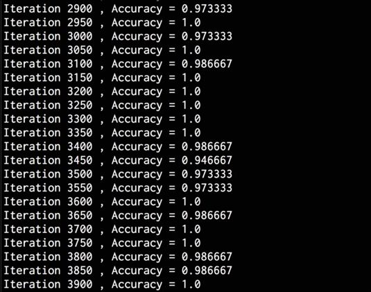
Now that you have the output, you can see that the accuracy of the Convolutional Neural Network far exceeds that of the simple neural network.
Editor: Yu Tengkai