Understanding Graph Neural Networks with PyTorch

Source: Algorithm Advancement


This article is approximately 4200 words long and is recommended for an 8-minute read. This article will introduce key parts of the "Graph Attention Networks" and implement the concepts proposed in the paper using PyTorch.

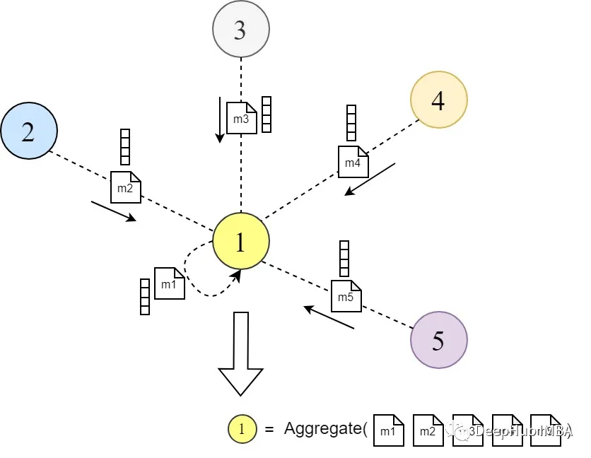
Graph Neural Networks (GNN) are a powerful class of neural networks that operate on graph-structured data. They learn node representations (embeddings) by aggregating information from the local neighborhood of nodes. This concept is referred to as “message passing” in the literature of graph representation learning.

Messages (embeddings) are passed between nodes in the graph through multiple GNN layers. Each node aggregates messages from its neighbors to update its representation. This process is repeated across layers, allowing nodes to obtain more informative representations that encode richer information about the graph. Major variants of GNNs include GraphSAGE[2], Graph Convolution Network[3], etc.

Graph Attention Networks (GAT)[1] are a classic type of GNN that is well-suited for getting started with GNN models. The main improvement is in the way messages are passed. They introduce a learnable attention mechanism that allows nodes to decide which neighboring nodes are more important when aggregating messages from local neighbors, rather than aggregating information from all neighbors with equal weight.

Graph Attention Networks outperform many other GNN models on tasks such as node classification, link prediction, and graph classification. They have also demonstrated state-of-the-art performance on several benchmark graph datasets.

In this article, we will introduce the key parts of the original “Graph Attention Networks” (by Veličković) paper and implement the concepts proposed in the paper using PyTorch to better grasp the GAT method.

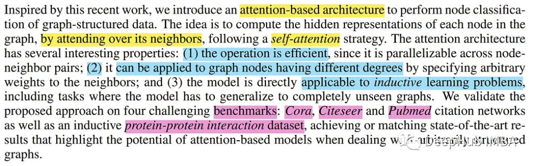
We will then compare the methods of the paper with some existing methods and point out their general similarities and differences, which is a common format in papers, so we won’t elaborate further.

Architecture of GAT

This section is the main part of this article, providing a detailed explanation of the architecture of Graph Attention Networks. To further illustrate, let’s assume the proposed architecture operates on a graph with N nodes (V = {V′}; i=1, …, N), where each node is represented by a vector h ^ (F elements), and there are arbitrary edges between nodes.

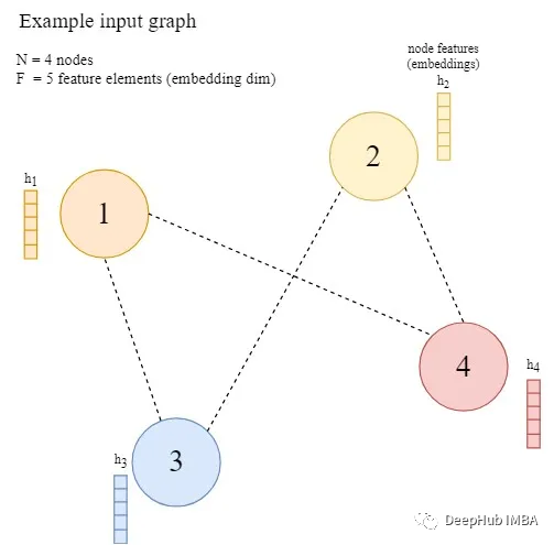
The author first describes the features of a single graph attention layer and how it operates (as it is the fundamental building block of graph attention networks). In general, a single GAT layer should take a graph with given node embeddings (representations) as input, propagate information to local neighboring nodes, and output updated node representations.

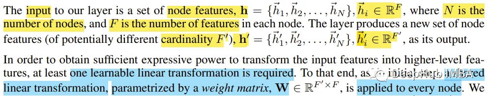
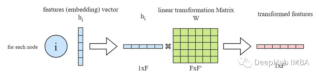
As mentioned, all input node feature vectors (h′) of the GAT layer undergo a linear transformation (i.e., multiplied by a weight matrix W). In PyTorch, this is typically done as follows:

 import torch from torch import nn
# in_features -> F and out_feature -> F'
in_features = ...
out_feature = ...
# instantiate the learnable weight matrix W (FxF')
W = nn.Parameter(torch.empty(size=(in_features, out_feature)))
# Initialize the weight matrix W
nn.init.xavier_normal_(W)
# multiply W and h (h is input features of all the nodes -> NxF matrix)
h_transformed = torch.mm(h, W)

After obtaining the transformed version of the input node features (embeddings), we jump to the end to see and understand what the final goal of the GAT layer is.

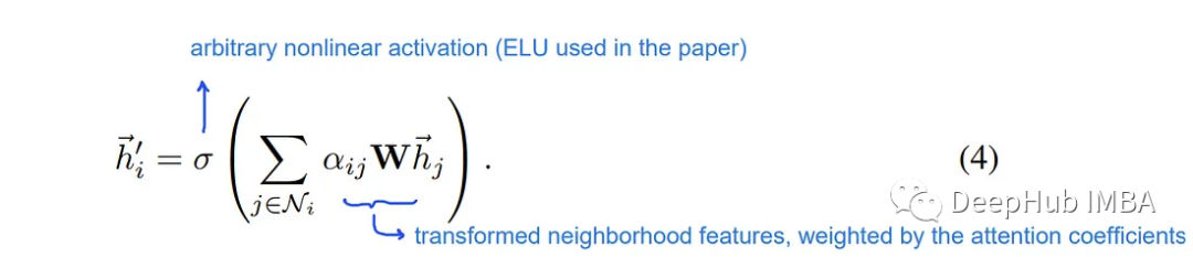
As described in the paper, at the end of the graph attention layer, for each node i, we need to obtain a new feature vector from its neighborhood that is more structurally and contextually aware.

This is accomplished by calculating the weighted sum of the features of neighboring nodes, followed by a nonlinear activation function σ. According to the Graph ML literature, this weighted sum is also referred to as the “aggregation” step in general GNN layer operations.

The weights α′ⱼ ∈ [0, 1] in the paper are learned and computed through an attention mechanism that indicates the importance of the features of neighbor j to node i during the message passing and aggregation process.

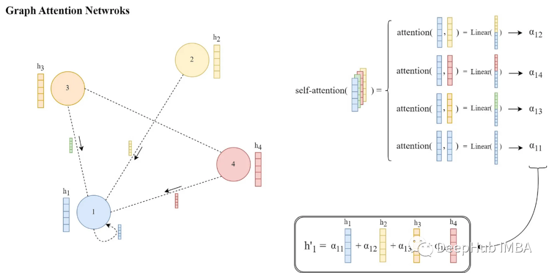
The calculation method for these attention weights α′ⱼ for each pair of nodes i and its neighbor j is as follows:

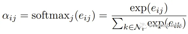
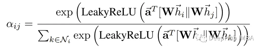
Where e ^ⱼ is the attention score, and after applying the Softmax function, the weights will be in the range of [0, 1], summing up to 1. Now, we calculate the attention scores e′ⱼ between each node i and its neighbor j ∈ N′ using the attention function a(…) as follows:

In the above diagram, || indicates the concatenation of two transformed node embeddings, and a is a learnable parameter vector of size 2 * F’ (twice the size of the transformed embedding). The expression a¹[Wh′|| Whⱼ] results from the dot (inner) product between a¹ (the transpose of vector a) and the concatenated transformed embeddings.

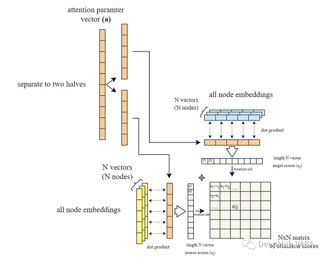
The entire operation is illustrated as follows:

In PyTorch, we adopt a slightly different approach. It is more efficient to compute all e′ⱼ for all pairs of nodes and then only select those corresponding to existing edges between nodes.

# instantiate the learnable attention parameter vector `a`
a = nn.Parameter(torch.empty(size=(2 * out_feature, 1)))
# Initialize the parameter vector `a`
nn.init.xavier_normal_(a)
# we obtained `h_transformed` in the previous code snippet
# calculating the dot product of all node embeddings
# and first half the attention vector parameters (corresponding to neighbor messages)
source_scores = torch.matmul(h_transformed, self.a[:out_feature, :])
# calculating the dot product of all node embeddings
# and second half the attention vector parameters (corresponding to target node)
target_scores = torch.matmul(h_transformed, self.a[out_feature:, :])
# broadcast add
e = source_scores + target_scores.T
e = self.leakyrelu(e)

The last part of the code snippet (# broadcast add) adds all pairwise source and target scores to obtain an NxN matrix containing all e′ⱼ scores (as shown in the diagram below).

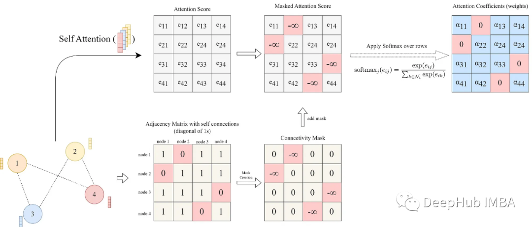
So far, we have assumed the graph is fully connected and we are calculating the attention scores for all possible pairs of nodes. However, in most cases, the graph cannot be fully connected. To address this issue, after applying the LeakyReLU activation to the attention scores, the attention scores are masked based on existing edges in the graph, meaning we only retain scores corresponding to existing edges.

This can be accomplished by assigning a large negative score (approximately -∞) to elements in the score matrix between nodes that do not have an edge, so that their corresponding attention weights become zero after softmax (remember the attention mask we mentioned earlier, it’s the same principle).

The attention mask here is implemented using the adjacency matrix of the graph. The adjacency matrix is an NxN matrix where there is a 1 at row i and column j if there is an edge between nodes i and j, and 0 elsewhere. Thus, we create a mask by assigning -∞ to the zero elements of the adjacency matrix and 0 elsewhere. We then add the mask to the score matrix and apply the softmax function on its rows.

connectivity_mask = -9e16 * torch.ones_like(e) # adj_mat is the N by N adjacency matrix
e = torch.where(adj_mat > 0, e, connectivity_mask) # masked attention scores
# attention coefficients are computed as a softmax over the rows
# for each column j in the attention score matrix e
attention = F.softmax(e, dim=-1)

Finally, according to the paper, after obtaining the attention scores and masking them with existing edges, we derive the attention weights α¹ⱼ by executing softmax over the rows of the score matrix.

We visualize the complete graph process as follows:

Finally, we compute the weighted sum of node embeddings:

# final node embeddings are computed as a weighted average of the features of its neighbors
h_prime = torch.matmul(attention, h_transformed)

The workflow and principles of a single attention head have been outlined above, and the paper also introduces the concept of multi-head attention, where all operations are performed through multiple parallel streams.

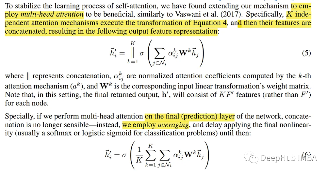
The multi-head attention and aggregation process is illustrated in the diagram below:

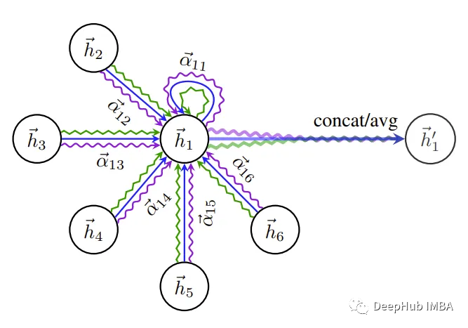
Node 1’s multi-head attention in its neighborhood (K = 3 heads), with different arrow styles and colors representing independent attention computations. The aggregated features from each head are concatenated or averaged to obtain h ‘.

To encapsulate the implementation in a more concise modular form (as a PyTorch module) and integrate the functionality of multi-head attention, the complete implementation of the Graph Attention layer is as follows:

import torch from torch import nn import torch.nn.functional as F
################################### GAT LAYER DEFINITION ###################################
class GraphAttentionLayer(nn.Module):
    def __init__(self, in_features: int, out_features: int, n_heads: int, concat: bool = False, dropout: float = 0.4, leaky_relu_slope: float = 0.2):
        super(GraphAttentionLayer, self).__init__()
        self.n_heads = n_heads # Number of attention heads
        self.concat = concat # whether to concatenate the final attention heads
        self.dropout = dropout # Dropout rate
        if concat: # concatenating the attention heads
            self.out_features = out_features # Number of output features per node
            assert out_features % n_heads == 0 # Ensure that out_features is a multiple of n_heads
            self.n_hidden = out_features // n_heads
        else: # averaging output over the attention heads (Used in the main paper)
            self.n_hidden = out_features
        # A shared linear transformation, parametrized by a weight matrix W is applied to every node
        # Initialize the weight matrix W
        self.W = nn.Parameter(torch.empty(size=(in_features, self.n_hidden * n_heads)))
        # Initialize the attention weights a
        self.a = nn.Parameter(torch.empty(size=(n_heads, 2 * self.n_hidden, 1)))
        self.leakyrelu = nn.LeakyReLU(leaky_relu_slope) # LeakyReLU activation function
        self.softmax = nn.Softmax(dim=1) # softmax activation function to the attention coefficients
        self.reset_parameters() # Reset the parameters

    def reset_parameters(self):
        nn.init.xavier_normal_(self.W)
        nn.init.xavier_normal_(self.a)
    def _get_attention_scores(self, h_transformed: torch.Tensor):
        source_scores = torch.matmul(h_transformed, self.a[:, :self.n_hidden, :])
        target_scores = torch.matmul(h_transformed, self.a[:, self.n_hidden:, :])
        # broadcast add
        # (n_heads, n_nodes, 1) + (n_heads, 1, n_nodes) = (n_heads, n_nodes, n_nodes)
        e = source_scores + target_scores.mT
        return self.leakyrelu(e)
    def forward(self, h: torch.Tensor, adj_mat: torch.Tensor):
        n_nodes = h.shape[0]
        # Apply linear transformation to node feature -> W h
        # output shape (n_nodes, n_hidden * n_heads)
        h_transformed = torch.mm(h, self.W)
        h_transformed = F.dropout(h_transformed, self.dropout, training=self.training)
        # splitting the heads by reshaping the tensor and putting heads dim first
        # output shape (n_heads, n_nodes, n_hidden)
        h_transformed = h_transformed.view(n_nodes, self.n_heads, self.n_hidden).permute(1, 0, 2)
        # getting the attention scores
        # output shape (n_heads, n_nodes, n_nodes)
        e = self._get_attention_scores(h_transformed)
        # Set the attention score for non-existent edges to -9e15 (MASKING NON-EXISTENT EDGES)
        connectivity_mask = -9e16 * torch.ones_like(e)
        e = torch.where(adj_mat > 0, e, connectivity_mask) # masked attention scores
        # attention coefficients are computed as a softmax over the rows
        # for each column j in the attention score matrix e
        attention = F.softmax(e, dim=-1)
        attention = F.dropout(attention, self.dropout, training=self.training)
        # final node embeddings are computed as a weighted average of the features of its neighbors
        h_prime = torch.matmul(attention, h_transformed)
        # concatenating/averaging the attention heads
        # output shape (n_nodes, out_features)
        if self.concat:
            h_prime = h_prime.permute(1, 0, 2).contiguous().view(n_nodes, self.out_features)
        else:
            h_prime = h_prime.mean(dim=0)
        return h_prime

Finally, we integrate all the above code into a complete GAT model:

class GAT(nn.Module):
    def __init__(self, in_features, n_hidden, n_heads, num_classes, concat=False, dropout=0.4, leaky_relu_slope=0.2):
        super(GAT, self).__init__()
        # Define the Graph Attention layers
        self.gat1 = GraphAttentionLayer(
            in_features=in_features, out_features=n_hidden, n_heads=n_heads,
            concat=concat, dropout=dropout, leaky_relu_slope=leaky_relu_slope
        )
        self.gat2 = GraphAttentionLayer(
            in_features=n_hidden, out_features=num_classes, n_heads=1,
            concat=False, dropout=dropout, leaky_relu_slope=leaky_relu_slope
        )
    def forward(self, input_tensor: torch.Tensor , adj_mat: torch.Tensor):
        # Apply the first Graph Attention layer
        x = self.gat1(input_tensor, adj_mat)
        x = F.elu(x) # Apply ELU activation function to the output of the first layer
        # Apply the second Graph Attention layer
        x = self.gat2(x, adj_mat)
        return F.softmax(x, dim=1) # Apply softmax activation function

Method Comparison

The authors compare GATs with several existing GNN methods/architectures:

• GATs can compute attention weights and perform local aggregation in parallel, making them computationally more efficient than some existing methods.

• GATs can assign different importance to a node’s neighbors when aggregating messages, which can achieve a leap in model capacity and improve interpretability.

• GAT does not consider the full neighborhood of nodes (does not require neighborhood sampling) and does not assume any ordering within the nodes.

• By setting the pseudo-coordinate function as u(x, y) = f(x)||f(y), GAT can be reformulated as a specific instance of MoNet (Monti et al., 2016), where f(x) represents the features of node x (possibly transformed by mlp), and || is concatenation; the weight function is wj(u) = softmax(MLP(u)).

Benchmarking

In the third part of the paper, the authors describe the benchmarks, datasets, and tasks used to evaluate GAT. They then present their evaluation results for the model.

The datasets used as benchmarks in the paper are divided into two types of tasks: transductive and inductive.

Inductive learning: This is a supervised learning task where the model is trained on a set of labeled training examples and is evaluated and tested on examples that were completely unobserved during training. This is a type of learning known as standard supervised learning.

Transductive learning: In this type of task, all data, including training, validation, and testing instances, is used during training. However, at each stage, the model only accesses the corresponding set of labels. This means that during training, the model is only trained using the loss generated by training instances and labels, but the test and validation features are used for message passing. This is primarily due to the structural and contextual information present in the examples.

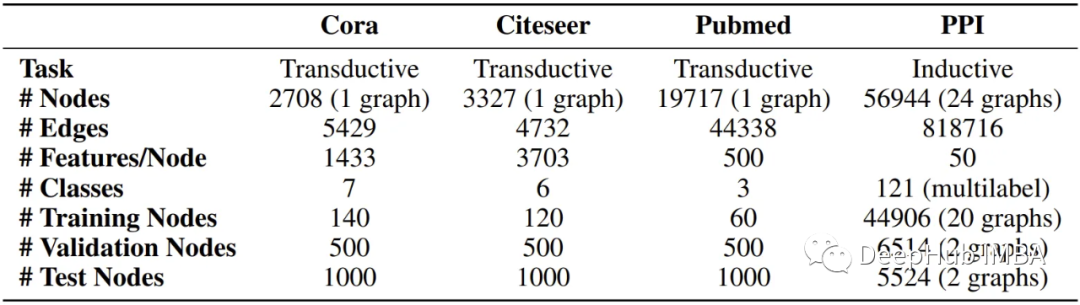
The paper uses four benchmark datasets to evaluate GATs, three of which correspond to transductive learning, while the other serves as an inductive learning task.

The transductive learning datasets, namely Cora, Citeseer, and Pubmed (Sen et al., 2008), are citation graphs where nodes are published documents, edges (connections) are their citations, and node features are the elements of a bag-of-words representation of the documents.

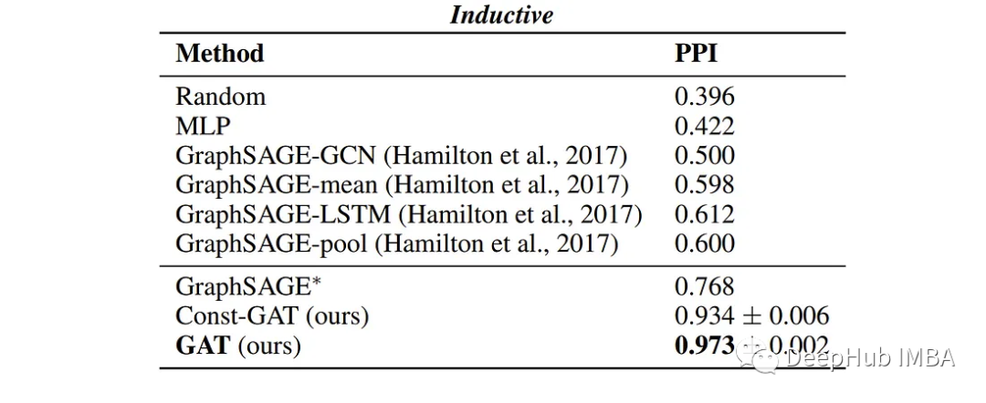
The inductive learning dataset is a protein-protein interaction (PPI) dataset containing graphs from different human tissues (Zitnik & Leskovec, 2017). A detailed description of the datasets is as follows:

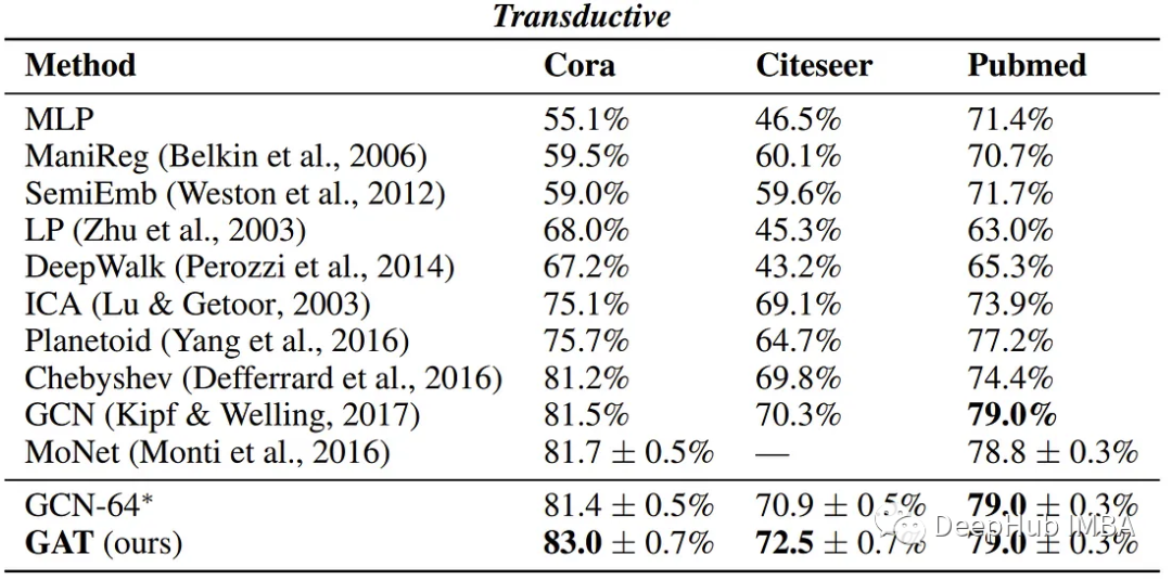
The authors report the following performance on the four benchmarks, showing comparable results of GATs with existing GNN methods.

Conclusion

By reading this article and trying out the code, I hope you can gain a solid understanding of how GATs work and how to apply them in practical scenarios.