
Source: DeepHub IMBA

This article is about 4900 words long and is recommended for a reading time of over 10 minutes.
Whether running on high-performance GPUs or edge devices, TorchDynamo adapts to provide optimal performance.
Optimizing model performance is crucial in deep learning, especially for applications that require fast execution and real-time inference. However, PyTorch often faces challenges in balancing dynamic graph execution with high performance. Traditional PyTorch optimization techniques have limited effectiveness when dealing with dynamic computation graphs, leading to longer training times and subpar model performance. TorchDynamo is a Just-In-Time (JIT) compiler designed for PyTorch that addresses this issue by intercepting Python code at runtime, optimizing it, and compiling it into efficient machine code. This article demonstrates the practical applications of TorchDynamo using synthetic datasets, including feature engineering, hyperparameter tuning, cross-validation, and evaluation metrics.
Introduction to TorchDynamo
TorchDynamo is a compiler frontend developed by the PyTorch team, aimed at automatically optimizing PyTorch programs to improve execution efficiency. TorchDynamo works by dynamically analyzing and transforming PyTorch code at runtime, then forwarding it to various backend compilers (such as TorchScript, TVM, Triton, etc.) to achieve performance enhancements.
Especially in applications requiring real-time execution, such as autonomous driving or financial forecasting, deep learning models demand fast execution. Traditional optimization techniques often require revisions when dealing with Python’s dynamic features, which is where TorchDynamo excels. It can capture computation graphs on the fly, optimizing for specific workloads and hardware applications, thereby reducing latency and increasing throughput.
Another notable feature of TorchDynamo is its ease of integration. Rewriting an entire codebase to integrate a new tool can be a daunting task. However, TorchDynamo requires minimal changes to existing PyTorch workflows. Its simplicity and powerful optimization capabilities make it a strong choice for experienced researchers and industry professionals.
Integrating TorchDynamo into existing PyTorch programs is relatively straightforward; you only need to import TorchDynamo into your program and use it to wrap the execution part of the model.
 import torch
import torchdynamo

# Define the model and optimizer
model = MyModel()
optimizer = torch.optim.Adam(model.parameters())

# Optimize the training process using TorchDynamo
def training_step(input, target):
    optimizer.zero_grad()
    output = model(input)
    loss = loss_fn(output, target)
    loss.backward()
    optimizer.step()
    return loss

# Wrap the training step with torchdynamo.optimize
optimized_training_step = torchdynamo.optimize(training_step)

# Training loop
for input, target in data_loader:
    loss = optimized_training_step(input, target)
How TorchDynamo Works
TorchDynamo dynamically captures computation graphs by tracing the execution of PyTorch code. This process involves understanding the dependencies and flow of the code, allowing it to identify opportunities for optimization. Once the computation graph is captured, TorchDynamo applies various optimization techniques. These techniques include operator fusion, which merges multiple operations into a single operation to reduce overhead, and improved memory management that minimizes data movement and efficiently reuses resources.
After optimizing the computation graph, TorchDynamo compiles it into efficient machine code. This compilation can target different backends, such as TorchScript or NVFuser, ensuring that the code runs optimally on the available hardware.
In the final execution phase, the optimizations applied can significantly improve performance compared to the original Python code. JIT compilation ensures that these optimizations are applied during runtime, making execution adapt to different workloads and input data.
Usage Example
Below we demonstrate a TorchDynamo example using a synthetic dataset, including feature engineering, hyperparameter tuning, cross-validation, prediction, and result interpretation.
import torch
import torch.nn as nn
import torch.optim as optim
import numpy as np
import pandas as pd
import matplotlib.pyplot as plt
from sklearn.model_selection import train_test_split, KFold
from sklearn.metrics import mean_squared_error, r2_score
from sklearn.preprocessing import StandardScaler
from torch import _dynamo as torchdynamo
from typing import List

# Generate synthetic dataset
np.random.seed(42)
torch.manual_seed(42)

# Feature engineering: create synthetic data
n_samples = 1000
n_features = 10
X = np.random.rand(n_samples, n_features)
y = X @ np.random.rand(n_features) + np.random.rand(n_samples) * 0.1  # Linear relation with noise

# Split data into train and test sets
X_train, X_test, y_train, y_test = train_test_split(X, y, test_size=0.2, random_state=42)

# Standardize the features
scaler = StandardScaler()
X_train = scaler.fit_transform(X_train)
X_test = scaler.transform(X_test)

# Convert to PyTorch tensors
X_train = torch.tensor(X_train, dtype=torch.float32)
y_train = torch.tensor(y_train, dtype=torch.float32).view(-1, 1)
X_test = torch.tensor(X_test, dtype=torch.float32)
y_test = torch.tensor(y_test, dtype=torch.float32).view(-1, 1)

# Define the model
class SimpleNN(nn.Module):
    def __init__(self, input_dim):
        super(SimpleNN, self).__init__()
        self.fc1 = nn.Linear(input_dim, 64)
        self.fc2 = nn.Linear(64, 32)
        self.fc3 = nn.Linear(32, 1)

    def forward(self, x):
        x = torch.relu(self.fc1(x))
        x = torch.relu(self.fc2(x))
        x = self.fc3(x)
        return x

# Hyperparameters
input_dim = X_train.shape[1]
learning_rate = 0.001
n_epochs = 100

# Initialize the model, loss function, and optimizer
model = SimpleNN(input_dim)
criterion = nn.MSELoss()
optimizer = optim.Adam(model.parameters(), lr=learning_rate)

# Define custom compiler
def my_compiler(gm: torch.fx.GraphModule, example_inputs: List[torch.Tensor]):
    print("my_compiler() called with FX graph:")
    gm.graph.print_tabular()
    return gm.forward  # return a python callable

@torchdynamo.optimize(my_compiler)
def train_and_evaluate(model, criterion, optimizer, X_train, y_train, X_test, y_test, n_epochs):
    # Training loop with K-Fold Cross-Validation
    kf = KFold(n_splits=5, shuffle=True, random_state=42)
    train_losses_per_epoch = np.zeros(n_epochs)
    val_losses_per_epoch = np.zeros(n_epochs)
    kf_count = 0

    for train_idx, val_idx in kf.split(X_train):
        X_kf_train, X_kf_val = X_train[train_idx], X_train[val_idx]
        y_kf_train, y_kf_val = y_train[train_idx], y_train[val_idx]

        for epoch in range(n_epochs):
            model.train()
            optimizer.zero_grad()
            y_pred_train = model(X_kf_train)
            train_loss = criterion(y_pred_train, y_kf_train)
            train_loss.backward()
            optimizer.step()

            model.eval()
            y_pred_val = model(X_kf_val)
            val_loss = criterion(y_pred_val, y_kf_val)

            train_losses_per_epoch[epoch] += train_loss.item()
            val_losses_per_epoch[epoch] += val_loss.item()

            kf_count += 1

    # Average losses over K-Folds
    train_losses_per_epoch /= kf_count
    val_losses_per_epoch /= kf_count

    # Evaluate on test data
    model.eval()
    y_pred_test = model(X_test)
    test_loss = criterion(y_pred_test, y_test).item()
    test_r2 = r2_score(y_test.detach().numpy(), y_pred_test.detach().numpy())

    return train_losses_per_epoch, val_losses_per_epoch, test_loss, test_r2

# Run training and evaluation with TorchDynamo optimization
train_losses, val_losses, test_loss, test_r2 = train_and_evaluate(model, criterion, optimizer, X_train, y_train, X_test, y_test, n_epochs)

# Print metrics
print(f"Test MSE: {test_loss:.4f}")
print(f"Test R^2: {test_r2:.4f}")

# Plot results
epochs = list(range(1, n_epochs + 1))
plt.plot(epochs, train_losses, label='Train Loss')
plt.plot(epochs, val_losses, label='Validation Loss')
plt.xlabel('Epochs')
plt.ylabel('Loss')
plt.legend()
plt.title('Training and Validation Loss')
plt.show()
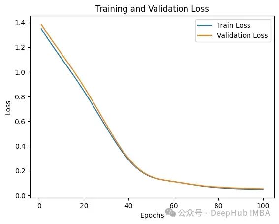
We defined a simple neural network with two hidden layers using PyTorch. The model employs K-Fold cross-validation to ensure robust performance. TorchDynamo is used to optimize the training loop. The model is evaluated on a separate test set, calculating metrics such as MSE and R².
The resulting training and validation losses are as follows:
We printed TorchDynamo-related content in the code using my_compiler; let’s take a look at what it contains:
my_compiler() called with FX graph:
opcode name target args kwargs
------------- ---------------------- ----------------------------------- ------------------------------------------------- --------
call_function train_losses_per_epoch <Wrapped function <original zeros>> (100,) {}
call_function val_losses_per_epoch <Wrapped function <original zeros>> (100,) {}
output output output ((train_losses_per_epoch, val_losses_per_epoch),) {}
my_compiler() called with FX graph:
opcode name target args kwargs
------------- ------------- ------------------------------------------------------- ----------------
placeholder l_x_ L_x_ () {}
call_module l__self___fc1 L__self___fc1 (l_x_,) {}
call_function x <built-in method relu of type object at 0x792eaaa81760> (l__self___fc1,) {}
call_module l__self___fc2 L__self___fc2 (x,) {}
call_function x_1 <built-in method relu of type object at 0x792eaaa81760> (l__self___fc2,) {}
call_module x_2 L__self___fc3 (x_1,) {}
output output output ((x_2,),) {}
my_compiler() called with FX graph:
opcode name target args kwargs
------------- ----------------------- -------------------------------------------------------- ------------------------------------------ --------------------------------
placeholder grad L_self_param_groups_0_params_0_grad () {}
placeholder grad_1 L_self_param_groups_0_params_1_grad () {}
placeholder grad_2 L_self_param_groups_0_params_2_grad () {}
placeholder grad_3 L_self_param_groups_0_params_3_grad () {}
placeholder grad_4 L_self_param_groups_0_params_4_grad () {}
placeholder grad_5 L_self_param_groups_0_params_5_grad () {}
get_attr param self___param_groups_0__params___0 () {}
get_attr param_1 self___param_groups_0__params___1 () {}
get_attr param_2 self___param_groups_0__params___2 () {}
get_attr param_3 self___param_groups_0__params___3 () {}
get_attr param_4 self___param_groups_0__params___4 () {}
get_attr param_5 self___param_groups_0__params___5 () {}
get_attr exp_avg self___state_list_L__self___state_keys____0___exp_avg () {}
get_attr exp_avg_1 self___state_list_L__self___state_keys____1___exp_avg () {}
get_attr exp_avg_2 self___state_list_L__self___state_keys____2___exp_avg () {}
get_attr exp_avg_3 self___state_list_L__self___state_keys____3___exp_avg () {}
get_attr exp_avg_4 self___state_list_L__self___state_keys____4___exp_avg () {}
get_attr exp_avg_5 self___state_list_L__self___state_keys____5___exp_avg () {}
get_attr exp_avg_sq self___state_list_L__self___state_keys____0___exp_avg_sq () {}
get_attr exp_avg_sq_1 self___state_list_L__self___state_keys____1___exp_avg_sq () {}
get_attr exp_avg_sq_2 self___state_list_L__self___state_keys____2___exp_avg_sq () {}
get_attr exp_avg_sq_3 self___state_list_L__self___state_keys____3___exp_avg_sq () {}
get_attr exp_avg_sq_4 self___state_list_L__self___state_keys____4___exp_avg_sq () {}
get_attr exp_avg_sq_5 self___state_list_L__self___state_keys____5___exp_avg_sq () {}
get_attr step_t self___state_list_L__self___state_keys____0___step () {}
get_attr step_t_2 self___state_list_L__self___state_keys____1___step () {}
get_attr step_t_4 self___state_list_L__self___state_keys____2___step () {}
get_attr step_t_6 self___state_list_L__self___state_keys____3___step () {}
get_attr step_t_8 self___state_list_L__self___state_keys____4___step () {}
get_attr step_t_10 self___state_list_L__self___state_keys____5___step () {}
call_function step <built-in function iadd> (step_t, 1) {}
call_method lerp_ lerp_ (exp_avg, grad, 0.09999999999999998) {}
call_method mul_ mul_ (exp_avg_sq, 0.999) {}
call_method conj conj (grad,) {}
call_method addcmul_ addcmul_ (mul_, grad, conj) {'value': 0.0010000000000000009}
call_function pow_1 <built-in function pow> (0.9, step) {}
call_function bias_correction1 <built-in function sub> (1, pow_1) {}
call_function pow_2 <built-in function pow> (0.999, step) {}
call_function bias_correction2 <built-in function sub> (1, pow_2) {}
call_function step_size <built-in function truediv> (0.001, bias_correction1) {}
call_method step_size_neg neg (step_size,) {}
call_method bias_correction2_sqrt sqrt (bias_correction2,) {}
call_method sqrt_1 sqrt (exp_avg_sq,) {}
call_function mul <built-in function mul> (bias_correction2_sqrt, step_size_neg) {}
call_function truediv_1 <built-in function truediv> (sqrt_1, mul) {}
call_function truediv_2 <built-in function truediv> (1e-08, step_size_neg) {}
call_method denom add_ (truediv_1, truediv_2) {}
call_method addcdiv_ addcdiv_ (param, exp_avg, denom) {}
call_function step_1 <built-in function iadd> (step_t_2, 1) {}
call_method lerp__1 lerp_ (exp_avg_1, grad_1, 0.09999999999999998) {}
call_method mul__1 mul_ (exp_avg_sq_1, 0.999) {}
call_method conj_1 conj (grad_1,) {}
call_method addcmul__1 addcmul_ (mul__1, grad_1, conj_1) {'value': 0.0010000000000000009}
call_function pow_3 <built-in function pow> (0.9, step_1) {}
call_function bias_correction1_1 <built-in function sub> (1, pow_3) {}
call_function pow_4 <built-in function pow> (0.999, step_1) {}
call_function bias_correction2_1 <built-in function sub> (1, pow_4) {}
call_function step_size_1 <built-in function truediv> (0.001, bias_correction1_1) {}
call_method step_size_neg_1 neg (step_size_1,) {}
call_method bias_correction2_sqrt_1 sqrt (bias_correction2_1,) {}
call_method sqrt_3 sqrt (exp_avg_sq_1,) {}
call_function mul_1 <built-in function mul> (bias_correction2_sqrt_1, step_size_neg_1) {}
call_function truediv_4 <built-in function truediv> (sqrt_3, mul_1) {}
call_function truediv_5 <built-in function truediv> (1e-08, step_size_neg_1) {}
call_method denom_1 add_ (truediv_4, truediv_5) {}
call_method addcdiv__1 addcdiv_ (param_1, exp_avg_1, denom_1) {}
call_function step_2 <built-in function iadd> (step_t_4, 1) {}
call_method lerp__2 lerp_ (exp_avg_2, grad_2, 0.09999999999999998) {}
call_method mul__2 mul_ (exp_avg_sq_2, 0.999) {}
call_method conj_2 conj (grad_2,) {}
call_method addcmul__2 addcmul_ (mul__2, grad_2, conj_2) {'value': 0.0010000000000000009}
call_function pow_5 <built-in function pow> (0.9, step_2) {}
call_function bias_correction1_2 <built-in function sub> (1, pow_5) {}
call_function pow_6 <built-in function pow> (0.999, step_2) {}
call_function bias_correction2_2 <built-in function sub> (1, pow_6) {}
call_function step_size_2 <built-in function truediv> (0.001, bias_correction1_2) {}
call_method step_size_neg_2 neg (step_size_2,) {}
call_method bias_correction2_sqrt_2 sqrt (bias_correction2_2,) {}
call_method sqrt_5 sqrt (exp_avg_sq_2,) {}
call_function mul_2 <built-in function mul> (bias_correction2_sqrt_2, step_size_neg_2) {}
call_function truediv_7 <built-in function truediv> (sqrt_5, mul_2) {}
call_function truediv_8 <built-in function truediv> (1e-08, step_size_neg_2) {}
call_method denom_2 add_ (truediv_7, truediv_8) {}
call_method addcdiv__2 addcdiv_ (param_2, exp_avg_2, denom_2) {}
call_function step_3 <built-in function iadd> (step_t_6, 1) {}
call_method lerp__3 lerp_ (exp_avg_3, grad_3, 0.09999999999999998) {}
call_method mul__3 mul_ (exp_avg_sq_3, 0.999) {}
call_method conj_3 conj (grad_3,) {}
call_method addcmul__3 addcmul_ (mul__3, grad_3, conj_3) {'value': 0.0010000000000000009}
call_function pow_7 <built-in function pow> (0.9, step_3) {}
call_function bias_correction1_3 <built-in function sub> (1, pow_7) {}
call_function pow_8 <built-in function pow> (0.999, step_3) {}
call_function bias_correction2_3 <built-in function sub> (1, pow_8) {}
call_function step_size_3 <built-in function truediv> (0.001, bias_correction1_3) {}
call_method step_size_neg_3 neg (step_size_3,) {}
call_method bias_correction2_sqrt_3 sqrt (bias_correction2_3,) {}
call_method sqrt_7 sqrt (exp_avg_sq_3,) {}
call_function mul_3 <built-in function mul> (bias_correction2_sqrt_3, step_size_neg_3) {}
call_function truediv_10 <built-in function truediv> (sqrt_7, mul_3) {}
call_function truediv_11 <built-in function truediv> (1e-08, step_size_neg_3) {}
call_method denom_3 add_ (truediv_10, truediv_11) {}
call_method addcdiv__3 addcdiv_ (param_3, exp_avg_3, denom_3) {}
call_function step_4 <built-in function iadd> (step_t_8, 1) {}
call_method lerp__4 lerp_ (exp_avg_4, grad_4, 0.09999999999999998) {}
call_method mul__4 mul_ (exp_avg_sq_4, 0.999) {}
call_method conj_4 conj (grad_4,) {}
call_method addcmul__4 addcmul_ (mul__4, grad_4, conj_4) {'value': 0.0010000000000000009}
call_function pow_9 <built-in function pow> (0.9, step_4) {}
call_function bias_correction1_4 <built-in function sub> (1, pow_9) {}
call_function pow_10 <built-in function pow> (0.999, step_4) {}
call_function bias_correction2_4 <built-in function sub> (1, pow_10) {}
call_function step_size_4 <built-in function truediv> (0.001, bias_correction1_4) {}
call_method step_size_neg_4 neg (step_size_4,) {}
call_method bias_correction2_sqrt_4 sqrt (bias_correction2_4,) {}
call_method sqrt_9 sqrt (exp_avg_sq_4,) {}
call_function mul_4 <built-in function mul> (bias_correction2_sqrt_4, step_size_neg_4) {}
call_function truediv_13 <built-in function truediv> (sqrt_9, mul_4) {}
call_function truediv_14 <built-in function truediv> (1e-08, step_size_neg_4) {}
call_method denom_4 add_ (truediv_13, truediv_14) {}
call_method addcdiv__4 addcdiv_ (param_4, exp_avg_4, denom_4) {}
call_function step_5 <built-in function iadd> (step_t_10, 1) {}
call_method lerp__5 lerp_ (exp_avg_5, grad_5, 0.09999999999999998) {}
call_method mul__5 mul_ (exp_avg_sq_5, 0.999) {}
call_method conj_5 conj (grad_5,) {}
call_method addcmul__5 addcmul_ (mul__5, grad_5, conj_5) {'value': 0.0010000000000000009}
call_function pow_11 <built-in function pow> (0.9, step_5) {}
call_function bias_correction1_5 <built-in function sub> (1, pow_11) {}
call_function pow_12 <built-in function pow> (0.999, step_5) {}
call_function bias_correction2_5 <built-in function sub> (1, pow_12) {}
call_function step_size_5 <built-in function truediv> (0.001, bias_correction1_5) {}
call_method step_size_neg_5 neg (step_size_5,) {}
call_method bias_correction2_sqrt_5 sqrt (bias_correction2_5,) {}
call_method sqrt_11 sqrt (exp_avg_sq_5,) {}
call_function mul_5 <built-in function mul> (bias_correction2_sqrt_5, step_size_neg_5) {}
call_function truediv_16 <built-in function truediv> (sqrt_11, mul_5) {}
call_function truediv_17 <built-in function truediv> (1e-08, step_size_neg_5) {}
call_method denom_5 add_ (truediv_16, truediv_17) {}
call_method addcdiv__5 addcdiv_ (param_5, exp_avg_5, denom_5) {}
output output output ((),) {}
my_compiler() called with FX graph:
opcode name target args kwargs
------------- ------------- ------------------------------------------------------- ----------------
placeholder s0 s0 () {}
placeholder l_x_ L_x_ () {}
call_module l__self___fc1 L__self___fc1 (l_x_,) {}
call_function x <built-in method relu of type object at 0x792eaaa81760> (l__self___fc1,) {}
call_module l__self___fc2 L__self___fc2 (x,) {}
call_function x_1 <built-in method relu of type object at 0x792eaaa81760> (l__self___fc2,) {}
call_module x_2 L__self___fc3 (x_1,) {}
output output output ((x_2,),) {}
The output of the FX graph indicates how the model’s structure and operations are organized:
Input 0 and L_x_ are placeholders representing input data.
The model passes the input through fully connected layers L__self___fc1, L__self___fc2, and L__self___fc3, which are the three layers of the neural network.
The ReLU activation function is applied after the first two layers.
The final output is produced after the third fully connected layer.
Conclusion
For researchers and engineers, training large and complex models can be time-consuming. TorchDynamo reduces this training time by optimizing computation graphs and accelerating execution, allowing for more iterations and experiments in a shorter time. In applications requiring real-time processing, such as video streaming or interactive AI systems, latency is critical. TorchDynamo’s ability to optimize and compile code at runtime ensures that these systems can operate smoothly and respond quickly to new data.
The flexibility of TorchDynamo in supporting multiple backends and hardware architectures makes it well-suited for deployment in various environments. Whether running on high-performance GPUs or edge devices, TorchDynamo adapts to provide optimal performance.
About Us
Data Pie THU, as a public account in data science, is backed by Tsinghua University Big Data Research Center, sharing cutting-edge data science and big data technology innovation research dynamics, continuously spreading data science knowledge, and striving to build a platform for gathering data talents, creating the strongest group in China’s big data.

Sina Weibo: @Data Pie THU
WeChat Video Account: Data Pie THU
Today’s Headline: Data Pie THU