
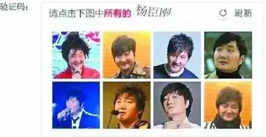
“Lookalikes” have always been a big joke in the entertainment industry.
If you run into Sun Nan, Yang Chenggang, Wang Daye… while buying a train ticket, face-blindness sufferers might as well give up going home and cry on the spot.
Of course, “lookalikes” are not unique to the entertainment industry; there are also some “similar-looking” professional terms in the AI field that confuse beginners, such as the “trio of similarities” we will explain tonight: DNN, RNN, CNN.
These three terms are actually three major algorithms widely used in the third generation of neural networks: DNN (Deep Neural Network), RNN (Recurrent Neural Network), and CNN (Convolutional Neural Network).
01
The Development of the Three Generations of Neural Networks
Before discussing the differences among these three, let’s briefly review what the first and second generations of neural networks are.
The first generation of neural networks, also known as perceptrons, was proposed around 1950. It has only two layers: an input layer and an output layer, mainly linear in structure. It cannot solve problems that are linearly inseparable and struggles with slightly more complex functions, such as the XOR operation.
To address the shortcomings of the first generation of neural networks, around 1980, Rumelhart, Williams, and others proposed the second generation of neural networks, the Multi-Layer Perceptron (MLP). Compared to the first generation, the second generation has multiple hidden layers between the input layers, allowing for some non-linear structures, thus overcoming the previous inability to simulate XOR logic.
The second generation of neural networks led scientists to discover that the number of layers directly determines its expressiveness in reality. However, as the number of layers increases, the optimization function tends to fall into local minima more easily. Due to the vanishing gradient problem, deep networks are often difficult to train and may perform worse than shallow networks.
In 2006, Hinton introduced the method of unsupervised pre-training to solve the vanishing gradient problem, making deep neural networks trainable, developing hidden layers to seven layers, thus truly giving neural networks “depth” and ushering in the wave of deep learning, marking the official rise of the third generation of neural networks.
02
The Three Most Common Algorithms in Deep Neural Networks
Having discussed the general development of the three generations of neural networks, let’s now look at the three major terms in the third generation of neural networks that often cause frustration: DNN, RNN, CNN.

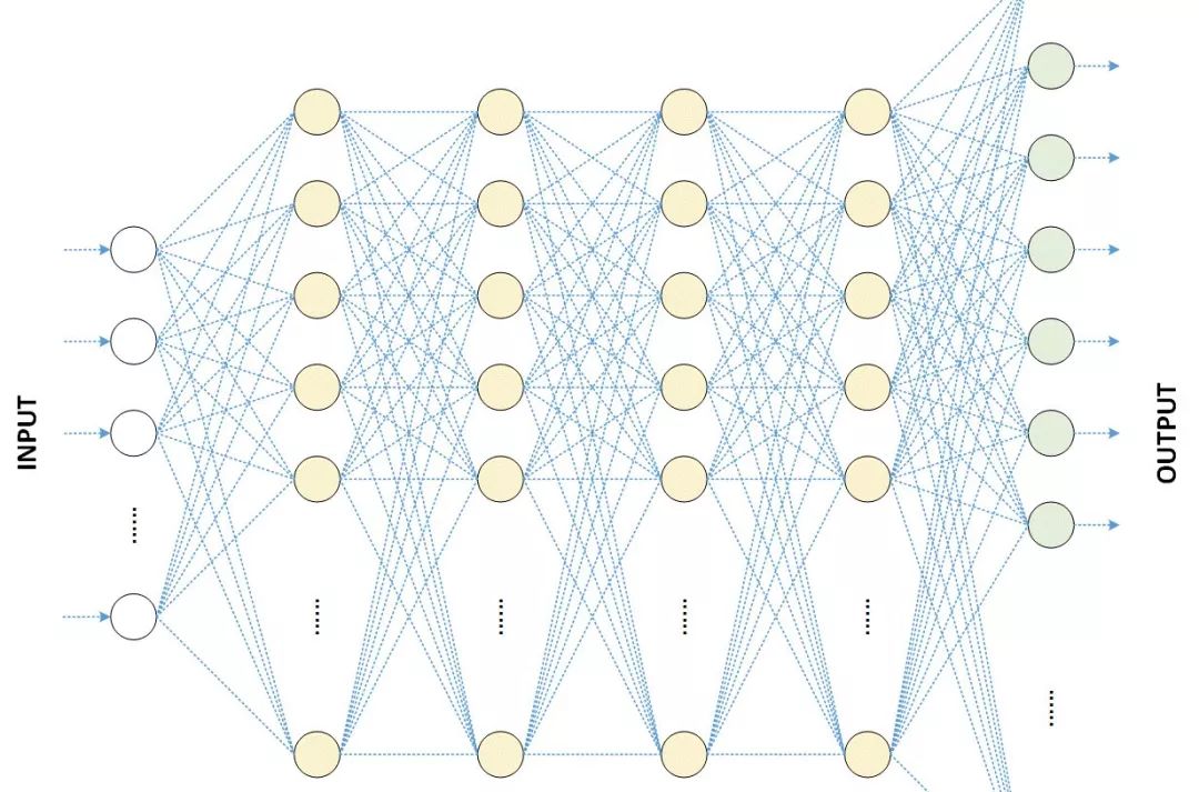
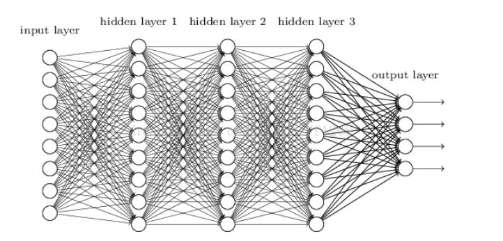
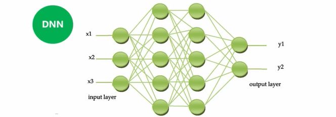
Structurally, DNN is not much different from traditional NN (Neural Network); the main difference is the increased number of layers and the resolution of the model’s trainability issue.
In simple terms, DNN has more hidden layers than NN, and these hidden layers have a huge impact, resulting in significant and miraculous effects.
However, the miraculous effects of the third generation of neural networks are not solely due to optimized model structures and advanced algorithms; the most important factor is the massive data generated with the popularization of mobile internet and the enhancement of machine computing power.
The “deep” in DNN refers to depth, but in deep learning, depth does not have a fixed definition or measurement standard. The number of hidden layers required to solve different problems varies. For example, in speech recognition, four layers may suffice, but for general image recognition, over 20 layers are usually needed.
The biggest problem with DNN is that it can only see pre-defined lengths of data, and its ability to represent sequential signals, such as speech and language, is still limited. Based on this, the RNN model, or Recurrent Neural Network, was proposed.

The fully connected DNN has an unsolvable problem: it cannot model changes in time series.
To address this need, the industry proposed the aforementioned Recurrent Neural Network (RNN).
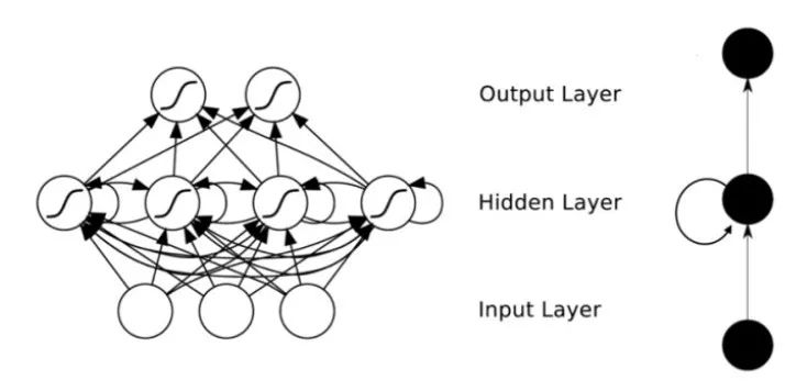
In a regular fully connected network, DNN’s hidden layer can only receive input from the previous layer at the current moment, while in RNN, the output of the neuron can directly affect itself in the next time segment. In other words, the hidden layer of the Recurrent Neural Network can receive input from both the previous layer and the input from the current hidden layer at the previous moment.
The significant implication of this change is that it gives the neural network a historical memory function, allowing it to theoretically access infinitely long historical information, making it very suitable for tasks like speech and language that have long-term dependencies.

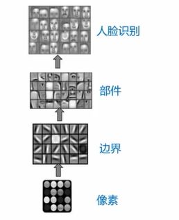
Convolutional Neural Networks are primarily proposed to simulate the human visual nervous system.
Taking CNN for facial recognition as an example, it first acquires some pixel information, then moves up to obtain boundary information, and then extracts facial component information including eyes, ears, eyebrows, and mouth, ultimately achieving facial recognition. This entire process is very similar to the human visual nervous system.
The structure of a Convolutional Neural Network still includes an input layer, hidden layers, and an output layer, where the hidden layers of the Convolutional Neural Network consist of three common types: convolutional layers, pooling layers, and fully connected layers. Next, we will focus on explaining the relevant knowledge points of convolution and pooling.
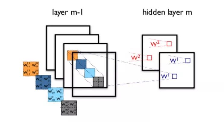
The function of the convolutional layer is to extract features from the input data, which contains multiple convolution kernels. The range of the original image covered by one convolution kernel is called the receptive field (weight sharing).
A single convolution operation (even with multiple convolution kernels) often extracts local features, making it difficult to extract global features; hence, further convolution calculations are needed on top of a layer of convolution, leading to multi-layer convolutions.
After feature extraction in the convolutional layer, the output feature map is passed to the pooling layer for feature selection and information filtering. The pooling layer contains predefined pooling functions, which replace the results of individual points in the feature map with statistics of their neighboring regions.
This pooling operation can somewhat overcome some rotations and minor local changes in images, making the feature representation more stable.
