
Essential Knowledge Delivered First-Hand
Essential Knowledge Delivered First-Hand
1. Introduction to CNN
CNN is a type of neural network that utilizes convolutional calculations. It can preserve the main features of a large image by reducing it to a smaller pixel image through convolutional calculations. This article specifically introduces the content from Professor Li Hongyi’s PPT.
1.1 Why CNN for Image
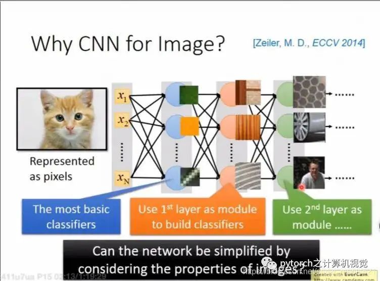
① Why introduce CNN?
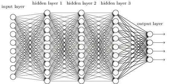
Image illustration: Given an image input into a fully connected neural network, the first hidden layer identifies whether there is green in the image, whether there is yellow, or whether there are diagonal stripes. The second hidden layer combines the outputs of the first hidden layer to achieve more complex functions. For example, if it sees a straight line + horizontal line, it indicates part of a box; if it sees brown + stripes, it indicates wood grain; if it sees diagonal stripes + green, it indicates part of a gray stripe. Based on the output of the second hidden layer, if a neuron sees a beehive, it will activate; if it sees a person, it will activate.
However, if we generally use a fully connected neural network, we will need many parameters. For example, if the input vector is 30,000 dimensions and the first hidden layer has 1,000 neurons, then the first hidden layer will require 30,000 * 1,000 parameters, leading to a huge data volume, resulting in low computational efficiency and accuracy. The introduction of CNN mainly addresses these issues by simplifying our neural network architecture. Some weights are unnecessary; CNN uses filtering methods to eliminate some unnecessary parameters and retain important ones for image processing.
② Why is it sufficient to use fewer parameters for image processing?
Three characteristics:
-
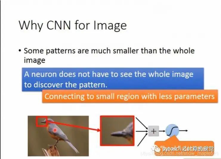
Most patterns are smaller than the entire image, so a neuron does not need to observe the entire image; it only needs to observe a small part of the image to find a desired pattern. For example, given an image, a neuron in the first hidden layer finds the bird’s beak, while another neuron finds the bird’s claws. As shown below, it only needs to look at the red box and does not need to observe the entire image to find the beak.
-
Different positions of the bird’s beak only need to train one parameter to recognize the beak; separate training is unnecessary.
-
We can use sub-sampling to reduce the image size; sub-sampling does not alter the target image.
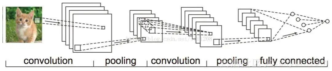
1.2 CNN Architecture Diagram

The first two properties in section 1.1 require convolutional calculations, while the last pooling layer processes them, which will be introduced in the next section.
1.3 Convolutional Layer
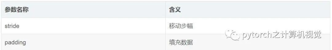
1.3.1 Important Parameters
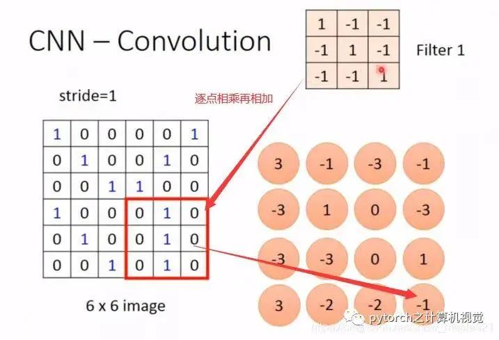
1.3.2 Convolution Calculation
The matrix convolution calculation is as follows:
The calculation is as follows: the input image has pixel values of 553, and after padding = 1, it forms pixel values of 773. The convolution kernel size is 333, with two convolution kernels and a stride of 2. Note that the depth of the convolution kernel must match the depth of the incoming pixel values. When the blue position scanned corresponds to the red position of the convolution kernel, the values are multiplied and summed to obtain the green position data.
The pixel number changes according to the formula: (n + 2p – f) / s = (5 + 2 – 3) / 2 + 1 = 3, resulting in 332 data. The pixel depth output after convolution equals the number of convolution kernels from the previous layer. The obtained result serves as the input value for the pooling layer.
The size of the convolution kernel is often chosen to be an odd number. The depth must match the pixel value depth of the previous layer. For example, the convolution kernel chosen in the animation is 3*3*3, while the output pixel value depth equals the number of convolution kernels used in this convolution. Do not confuse this point.
1.3.3 Relationship Between Convolutional Layer and Fully Connected Layer
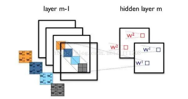
In fact, convolution is about removing some weights from the fully connected layer. The output result calculated by the convolutional layer is actually the output of the hidden layer of the fully connected layer. As shown in the figure:
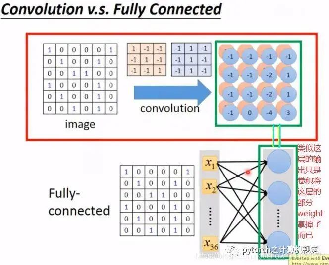
Convolution does not consider all features of the input, only those relevant to the features passed through the filter. For example, a 6*6 image unfolds into 36 pixels, and the next layer only relates to 9 pixels of the input layer, without connecting to all, thus using very few parameters. The specific diagram is as follows:
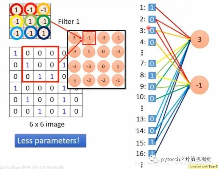
From the above figure, it can also be seen that the calculations for 3 and -1 do not require different weights like in a fully connected network, and the weights for these calculations are the same, which is known as parameter sharing.
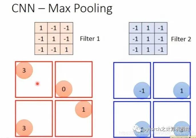
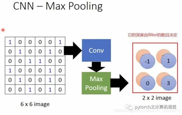
1.4 Pooling Layer
Based on the matrix after the previous convolution calculation, pooling is then performed (merging four values within a frame into one value, taking the maximum or average), as shown in the figure:
1.5 Applications
The PyTorch framework is mainly used to introduce convolutional neural networks.
Source code:
torch.nn.Conv2d(
    in_channels: int, # Number of input image channels
    out_channels: int, # Number of output channels produced by the convolution
    kernel_size: Union[T, Tuple[T, T]], # Size of the convolution kernel
    stride: Union[T, Tuple[T, T]] = 1, # Default stride: 1
    padding: Union[T, Tuple[T, T]] = 0, # Default padding: 0 added to both sides of the input
    dilation: Union[T, Tuple[T, T]] = 1, # Default spacing between kernel elements: 1
    groups: int = 1, # Number of blocked connections from input channels to output channels, default: 1
    # groups: controls connections between input and output, input and output channels must be divisible by the group
    # When groups=1: all inputs are handed to all outputs
    # When groups=2: equivalent to two convolutional layers, one seeing half of the input channels and producing half of the output channels, merging the two
    # When groups=in_channels: each channel has its own set of filters, with size out_channel/in_channel
    bias: bool = True, # Adds learnable bias to the output, default: true
    padding_mode: str = 'zeros')
# Note: kernel_size, stride, padding, dilation parameter types can be int or tuple. When tuple, the first int is height dimension, the second is width dimension. When a single int, height and width values are the same.

# Square kernel and equal stride
m = nn.Conv2d(16, 33, 3, stride=2)
# Non-square kernel and unequal stride and padding
m = nn.Conv2d(16, 33, (3, 5), stride=(2, 1), padding=(4, 2))
# Non-square kernel and unequal stride and padding and dilation
m = nn.Conv2d(16, 33, (3, 5), stride=(2, 1), padding=(4, 2), dilation=(3, 1))
input = torch.randn(20, 16, 50, 100)
output = m(input)
Application: Here, VGG16 is used, and the torchsummary library of PyTorch is introduced, which can print out the network model, for example:
import torchvision.models as models
import torch.nn as nn
import torch
from torchsummary import summary

device = torch.device('cuda' if torch.cuda.is_available() else 'cpu')

model = models.vgg16(pretrained=True).to(device)
print(model)
Output:
VGG(
  (features): Sequential(
    (0): Conv2d(3, 64, kernel_size=(3, 3), stride=(1, 1), padding=(1, 1))
    (1): ReLU(inplace)
    (2): Conv2d(64, 64, kernel_size=(3, 3), stride=(1, 1), padding=(1, 1))
    (3): ReLU(inplace)
    (4): MaxPool2d(kernel_size=2, stride=2, padding=0, dilation=1, ceil_mode=False)
    (5): Conv2d(64, 128, kernel_size=(3, 3), stride=(1, 1), padding=(1, 1))
    (6): ReLU(inplace)
    (7): Conv2d(128, 128, kernel_size=(3, 3), stride=(1, 1), padding=(1, 1))
    (8): ReLU(inplace)
    (9): MaxPool2d(kernel_size=2, stride=2, padding=0, dilation=1, ceil_mode=False)
    (10): Conv2d(128, 256, kernel_size=(3, 3), stride=(1, 1), padding=(1, 1))
    (11): ReLU(inplace)
    (12): Conv2d(256, 256, kernel_size=(3, 3), stride=(1, 1), padding=(1, 1))
    (13): ReLU(inplace)
    (14): Conv2d(256, 256, kernel_size=(3, 3), stride=(1, 1), padding=(1, 1))
    (15): ReLU(inplace)
    (16): MaxPool2d(kernel_size=2, stride=2, padding=0, dilation=1, ceil_mode=False)
    (17): Conv2d(256, 512, kernel_size=(3, 3), stride=(1, 1), padding=(1, 1))
    (18): ReLU(inplace)
    (19): Conv2d(512, 512, kernel_size=(3, 3), stride=(1, 1), padding=(1, 1))
    (20): ReLU(inplace)
    (21): Conv2d(512, 512, kernel_size=(3, 3), stride=(1, 1), padding=(1, 1))
    (22): ReLU(inplace)
    (23): MaxPool2d(kernel_size=2, stride=2, padding=0, dilation=1, ceil_mode=False)
    (24): Conv2d(512, 512, kernel_size=(3, 3), stride=(1, 1), padding=(1, 1))
    (25): ReLU(inplace)
    (26): Conv2d(512, 512, kernel_size=(3, 3), stride=(1, 1), padding=(1, 1))
    (27): ReLU(inplace)
    (28): Conv2d(512, 512, kernel_size=(3, 3), stride=(1, 1), padding=(1, 1))
    (29): ReLU(inplace)
    (30): MaxPool2d(kernel_size=2, stride=2, padding=0, dilation=1, ceil_mode=False)
  )
  (classifier): Sequential(
    (0): Linear(in_features=25088, out_features=4096, bias=True)
    (1): ReLU(inplace)
    (2): Dropout(p=0.5)
    (3): Linear(in_features=4096, out_features=4096, bias=True)
    (4): ReLU(inplace)
    (5): Dropout(p=0.5)
    (6): Linear(in_features=4096, out_features=1000, bias=True)
  )
)
model.classifier = nn.Sequential(
    *list(model.classifier.children())[:-1])    # remove last fc layer
print(model)
summary(model,(3,224,224))
Output:
----------------------------------------------------------------
        Layer (type)               Output Shape         Param #
================================================================
            Conv2d-1         [-1, 64, 224, 224]           1,792
              ReLU-2         [-1, 64, 224, 224]               0
            Conv2d-3         [-1, 64, 224, 224]          36,928
              ReLU-4         [-1, 64, 224, 224]               0
         MaxPool2d-5         [-1, 64, 112, 112]               0
            Conv2d-6        [-1, 128, 112, 112]          73,856
              ReLU-7        [-1, 128, 112, 112]               0
            Conv2d-8        [-1, 128, 112, 112]         147,584
              ReLU-9        [-1, 128, 112, 112]               0
        MaxPool2d-10          [-1, 128, 56, 56]               0
           Conv2d-11          [-1, 256, 56, 56]         295,168
             ReLU-12          [-1, 256, 56, 56]               0
           Conv2d-13          [-1, 256, 56, 56]         590,080
             ReLU-14          [-1, 256, 56, 56]               0
           Conv2d-15          [-1, 256, 56, 56]         590,080
             ReLU-16          [-1, 256, 56, 56]               0
        MaxPool2d-17          [-1, 256, 28, 28]               0
           Conv2d-18          [-1, 512, 28, 28]       1,180,160
             ReLU-19          [-1, 512, 28, 28]               0
           Conv2d-20          [-1, 512, 28, 28]       2,359,808
             ReLU-21          [-1, 512, 28, 28]               0
           Conv2d-22          [-1, 512, 28, 28]       2,359,808
             ReLU-23          [-1, 512, 28, 28]               0
        MaxPool2d-24          [-1, 512, 14, 14]               0
           Conv2d-25          [-1, 512, 14, 14]       2,359,808
             ReLU-26          [-1, 512, 14, 14]               0
           Conv2d-27          [-1, 512, 14, 14]       2,359,808
             ReLU-28          [-1, 512, 14, 14]               0
           Conv2d-29          [-1, 512, 14, 14]       2,359,808
             ReLU-30          [-1, 512, 14, 14]               0
        MaxPool2d-31            [-1, 512, 7, 7]               0
           Linear-32                 [-1, 4096]     102,764,544
             ReLU-33                 [-1, 4096]               0
          Dropout-34                 [-1, 4096]               0
           Linear-35                 [-1, 4096]      16,781,312
             ReLU-36                 [-1, 4096]               0
          Dropout-37                 [-1, 4096]               0
================================================================
Total params: 134,260,544
Trainable params: 134,260,544
Non-trainable params: 0
----------------------------------------------------------------
Input size (MB): 0.57
Forward/backward pass size (MB): 218.58
Params size (MB): 512.16
Estimated Total Size (MB): 731.32
----------------------------------------------------------------
2. Introduction to RNN
2.1 Introduction
Every ticketing system has a slot filling function; some slots are for Destination, and some are for time of arrival. The system needs to know which words belong to which slot; for example:
I would like to arrive Taipei on November 2nd;
Here, Taipei is the Destination, and November 2nd is the time of arrival;
Using a regular neural network, the word Taipei is input into the network, but before that, it must be converted into a vector representation. There are many ways to represent it; here we use: 1-of-N Encoding, represented as follows:
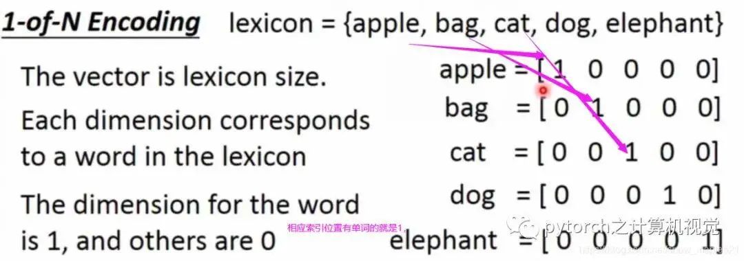
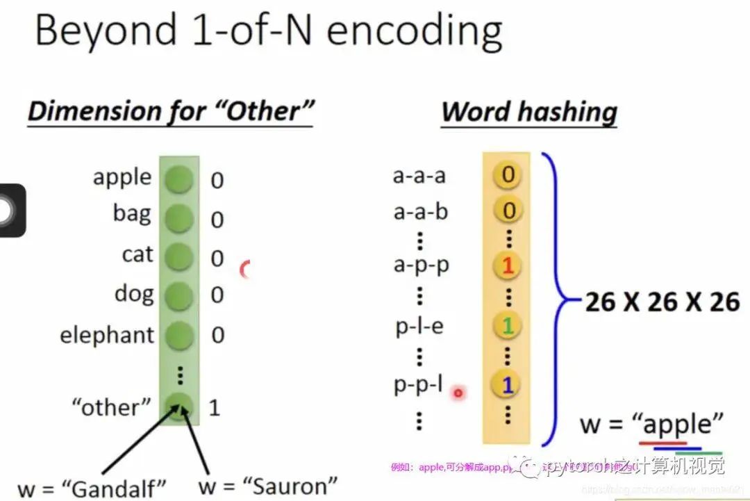
Other word vector representations are as follows:
However, if the following situation occurs, the system will make an error.

Question: What to do? Sometimes when inputting Taipei, the output probability for destination is high, and sometimes when inputting Taipei, the output probability for departure is high?
Answer: At this point, our network needs to have “memory” to remember the previously input data. For example, when Taipei is a destination, it sees arrive; when Taipei is a departure, it sees leave. This type of memory network is called a Recurrent Neural Network (RNN).
2.2 Introduction to RNN
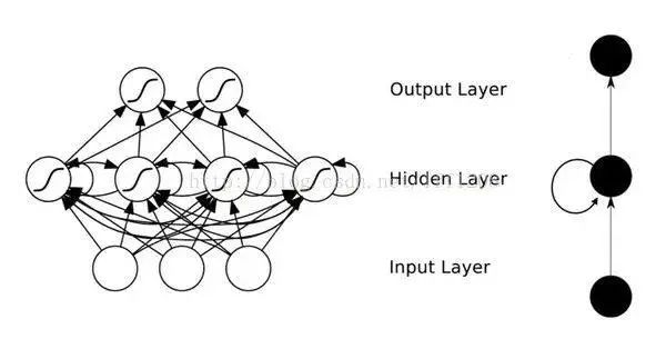
The output of the hidden layer of RNN will be stored in memory, and when the next data is input, the stored previous output will be used. The illustration is as follows:
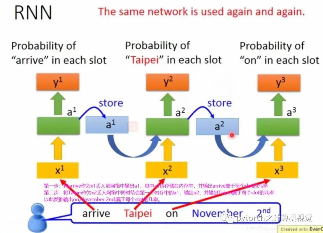
In the figure, the same weights are represented by the same color. Of course, the hidden layer can have many layers; the RNN introduced above is the simplest. The next section will introduce the enhanced version, LSTM.
2.3 LSTM of RNN
The commonly used memory is Long Short-Term Memory.
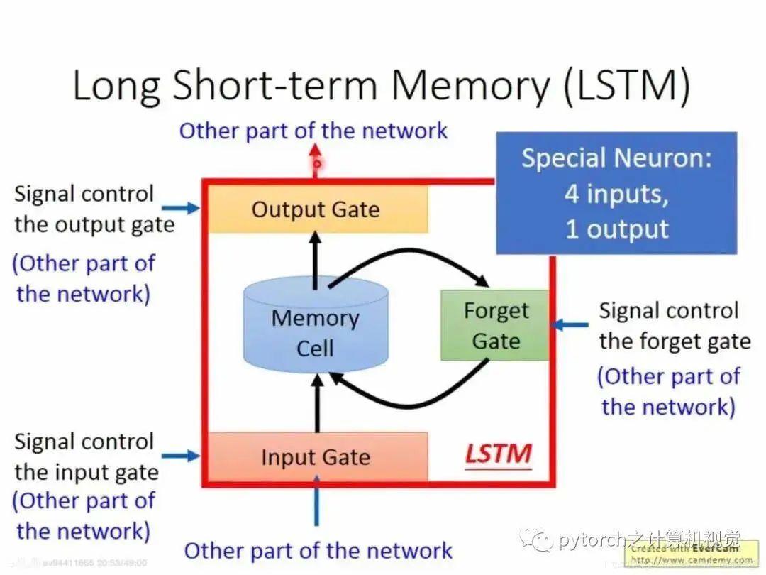
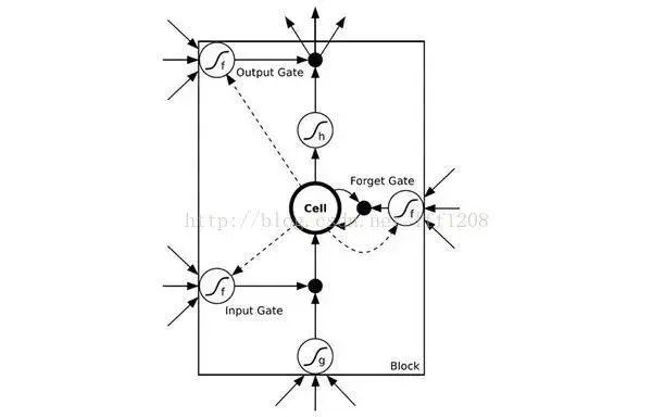
When external information needs to be input into memory, a “gate”—input gate is required, and when to open and close the input gate is learned by the neural network. Similarly, the output gate is also learned by the neural network, and the same goes for the forget gate.
Therefore, LSTM has four inputs and one output. The simplified diagram is as follows:
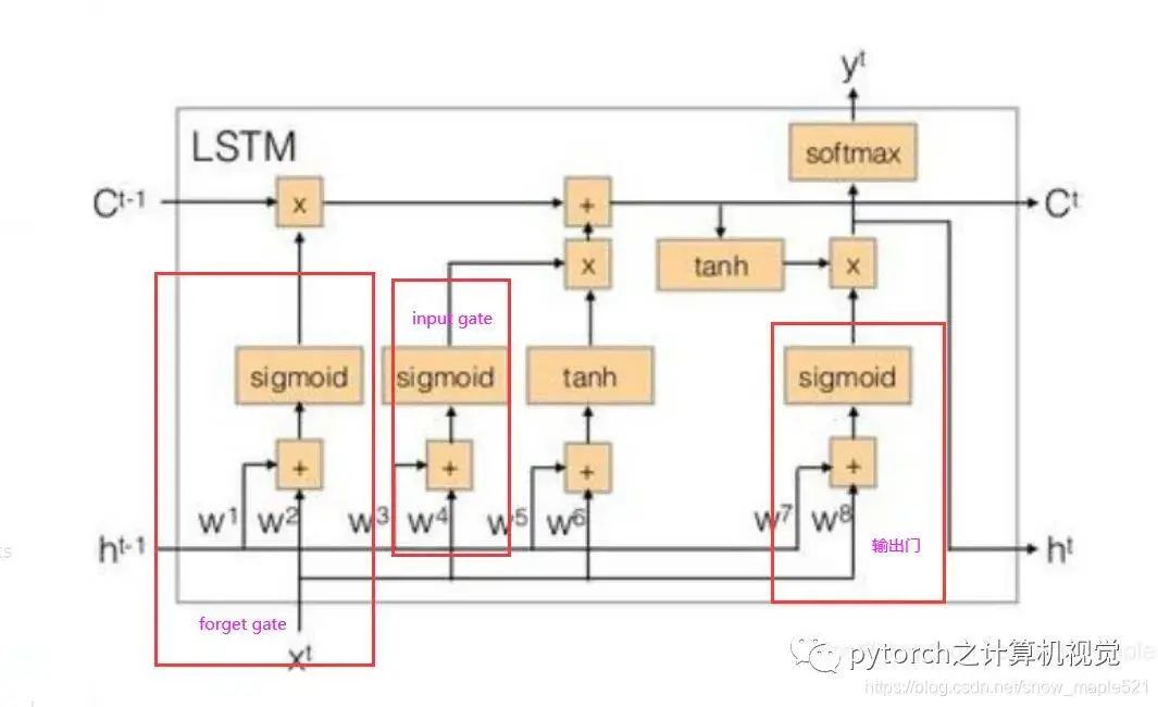
The formulas are as follows:
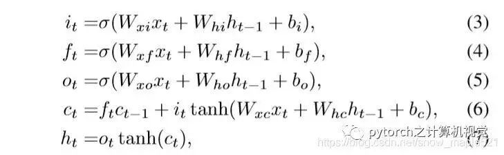
2.4 Example of LSTM
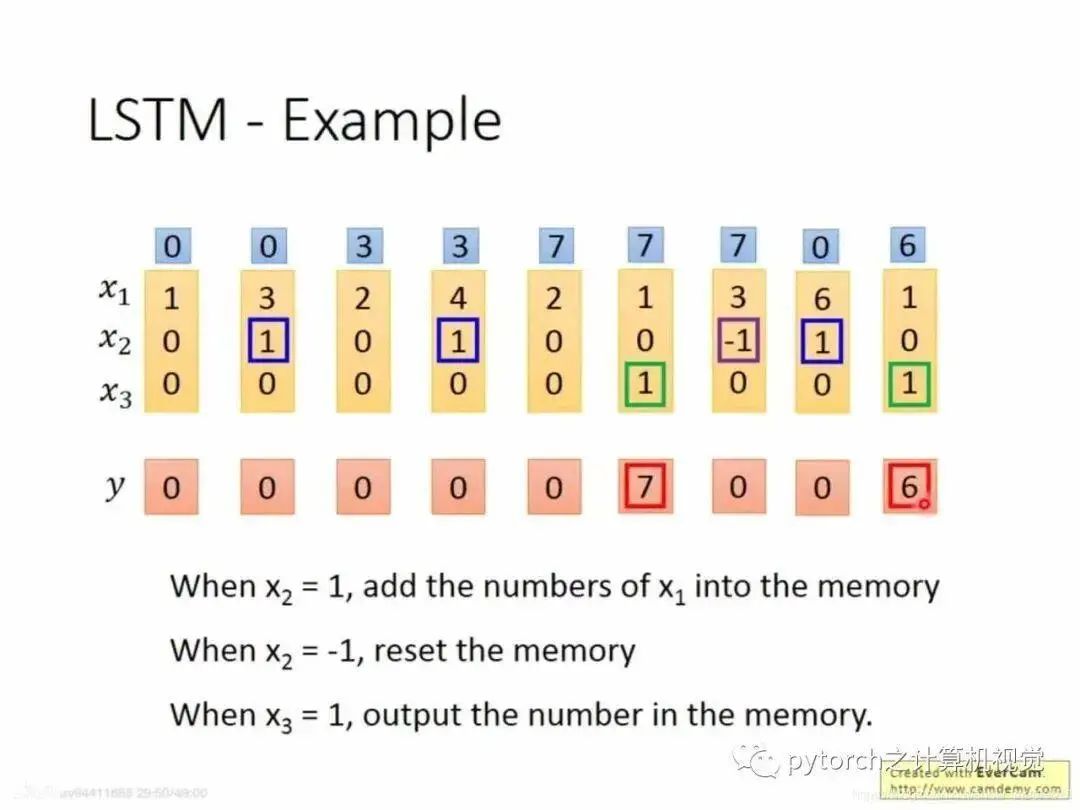
In the figure, x2 = 1 sends x1 into memory; if x2 = -1, it clears the memory value; if x3 = 1, it outputs the data from memory. In the above figure, in the first column, x2 = 0 does not send to memory; in the second column, x2 = 1 sends x1 = 3 into memory (note that the data in memory is cumulative, for example, in the fourth column, x2 = 1, at this time x1 = 4, memory = 3, so the total is 7). In the fifth column, x3 = 1, so it outputs the value from memory, which is 7.
Combining the LSTM simplified diagram:
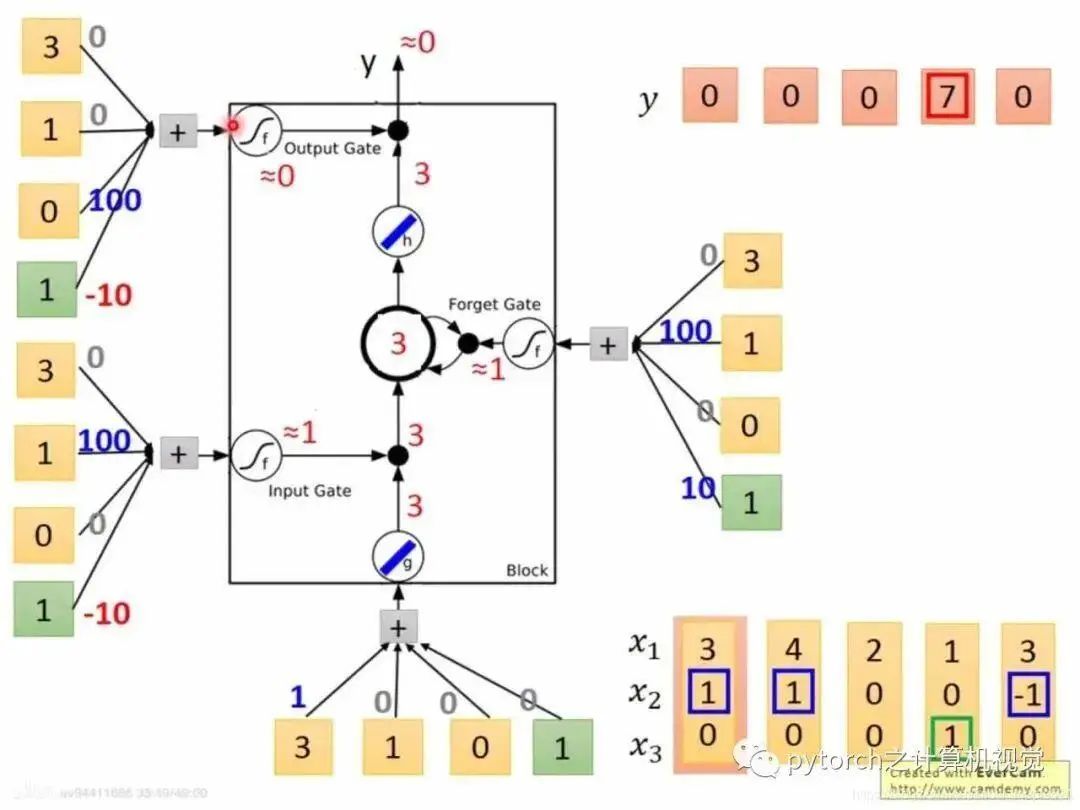
Assuming the first column input is: x1=3, x2=1, x3=0 steps: g—Tanh: x1w1+x2w2+x3w3 = 3f—sigmoid: x1w1+x2w2+x3w3=90 sigmoid after=1. After calculating f and g, input gate = 3*1=3, forget gate = 1, indicating no need to clear, x3 = 0, indicating the output gate is locked, so the output is still 0.
2.5 Practical Implementation of LSTM
The LSTM network is encapsulated in PyTorch, and can be used directly with nn.LSTM, for example:
class QstEncoder(nn.Module):

    def __init__(self, qst_vocab_size, word_embed_size, embed_size, num_layers, hidden_size):

        super(QstEncoder, self).__init__()
        self.word2vec = nn.Embedding(qst_vocab_size, word_embed_size)
        self.tanh = nn.Tanh()
        self.lstm = nn.LSTM(word_embed_size, hidden_size, num_layers)
        self.fc = nn.Linear(2*num_layers*hidden_size, embed_size)     # 2 for hidden and cell states
    def forward(self, question):

        qst_vec = self.word2vec(question)                             # [batch_size, max_qst_length=30, word_embed_size=300]
        qst_vec = self.tanh(qst_vec)
        qst_vec = qst_vec.transpose(0, 1)                             # [max_qst_length=30, batch_size, word_embed_size=300]
        _, (hidden, cell) = self.lstm(qst_vec)                        # [num_layers=2, batch_size, hidden_size=512]
        qst_feature = torch.cat((hidden, cell), 2)                    # [num_layers=2, batch_size, 2*hidden_size=1024]
        qst_feature = qst_feature.transpose(0, 1)                     # [batch_size, num_layers=2, 2*hidden_size=1024]
        qst_feature = qst_feature.reshape(qst_feature.size()[0], -1)  # [batch_size, 2*num_layers*hidden_size=2048]
        qst_feature = self.tanh(qst_feature)
        qst_feature = self.fc(qst_feature)                            # [batch_size, embed_size]

        return qst_feature
3. Differences Between CNN and RNN
The differences between CNN and RNN are linked as follows, quoting the summary from this blog author, (https://blog.csdn.net/lff1208/article/details/77717149) as detailed below.
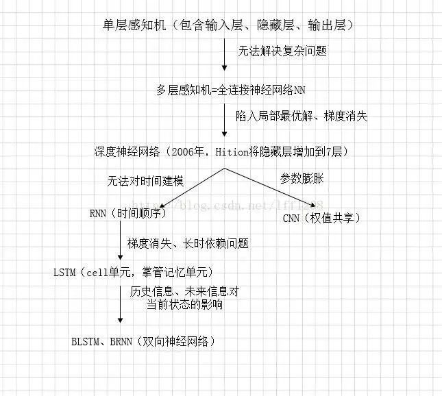
DNN Formation
To overcome the gradient disappearance, functions such as ReLU and maxout have replaced sigmoid, forming the basic form of DNN today. The structure is similar to a multilayer perceptron, as shown in the figure below:
We see that in the structure of fully connected DNN, lower-layer neurons can connect to all upper-layer neurons, leading to an explosion in the number of parameters. Suppose the input is an image with a pixel size of 1K*1K, and the hidden layer has 1M nodes; just this layer would require 10^12 weights to train, which not only easily leads to overfitting but also easily falls into local optima.
CNN Formation
Due to the inherent local patterns in images (such as eyes, noses, mouths in faces, etc.), the convolutional neural network (CNN) is introduced by combining image processing and neural networks. CNN links upper and lower layers through convolutional kernels, where the same convolutional kernel is shared across all images, and the original positional relationships are preserved after convolution operations on the images.
To illustrate the structure of convolutional neural networks simply, suppose we need to recognize a color image that has four channels ARGB (transparency and red, green, blue, corresponding to four identical-sized images). Suppose the convolution kernel size is 100*100, and we use 100 convolution kernels from w1 to w100 (intuitively, each convolution kernel should learn different structural features).
Using w1 to perform convolution operations on the ARGB image can yield the first image of the hidden layer; the upper left pixel of this hidden layer image is the weighted sum of the pixels in the upper left 100*100 area of the four input images, and so on.
Similarly, considering other convolution kernels, the hidden layer corresponds to 100 “images.” Each image corresponds to the response of different features in the original image. Following this structure, CNN also includes operations like max-pooling to further improve robustness.
It is noted that the last layer is actually a fully connected layer. In this example, we see that the parameters from the input layer to the hidden layer instantly drop to 100*100*100=10^6! This allows us to obtain a good model with existing training data. The question posed by the user regarding image recognition is precisely due to the characteristic of the CNN model limiting the number of parameters and exploiting local structures. Following the same logic, utilizing local information in speech spectrum structures, CNN can also be applied in speech recognition.
RNN Formation
DNN cannot model changes over time series. However, the temporal order of sample appearances is very important for applications like natural language processing, speech recognition, and handwriting recognition. To meet this demand, another neural network structure called Recurrent Neural Network (RNN) was introduced.
In a regular fully connected network or CNN, the signals of neurons in each layer can only propagate to the upper layer, and the processing of samples at each moment is independent, hence they are also called feed-forward neural networks. In RNN, the output of neurons can directly affect themselves at the next time period, that is, the input of the i-th layer neuron at time m includes not only the output of the (i-1) layer neuron at that moment but also its own output at (m-1) moment! This can be represented in a diagram as follows:
For convenience in analysis, the following diagram is expanded over time periods:
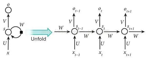
The final result O(t+1) of the network at time (t+1) is the result of that moment’s input and all historical influences! This achieves the purpose of modeling time series. RNN can be viewed as a neural network that transmits over time, where its depth is the length of time! Just as we mentioned above, the “gradient disappearance” phenomenon will also occur, but this time it happens along the time axis.
Thus, RNN faces the problem of long-term dependencies that it cannot solve. To address this, LSTM (Long Short-Term Memory) was proposed, which enables memory functionality over time through cell gates and prevents gradient disappearance. The structure of LSTM units is shown in the diagram below:
In addition to DNN, CNN, RNN, ResNet (Deep Residual), LSTM, there are many other neural network structures. For instance, in sequence signal analysis, if I can predict the future, it will also be helpful for recognition. Therefore, bidirectional RNN and bidirectional LSTM have been developed, which utilize both historical and future information.
In fact, regardless of which network, they are often used in combination in practical applications. For example, CNN and RNN often connect a fully connected layer before the output, making it difficult to determine which network belongs to which category. It is not hard to imagine that as the popularity of deep learning continues, more flexible combinations and more network structures will be developed.
In summary:
Download 1: OpenCV-Contrib Extension Module Chinese Version Tutorial

Reply with "Extension Module Chinese Tutorial" in the backend of the "Beginner's Guide to Vision" public account to download the first OpenCV extension module tutorial in Chinese, covering installation of extension modules, SFM algorithms, stereo vision, target tracking, biological vision, super-resolution processing, and more than twenty chapters of content.

Download 2: Python Vision Practical Project 52 Lectures

Reply with "Python Vision Practical Project" in the backend of the "Beginner's Guide to Vision" public account to download 31 practical vision projects including image segmentation, mask detection, lane line detection, vehicle counting, eyeliner addition, license plate recognition, character recognition, emotion detection, text content extraction, face recognition, etc., to aid in quickly learning computer vision.

Download 3: OpenCV Practical Projects 20 Lectures

Reply with "OpenCV Practical Projects 20 Lectures" in the backend of the "Beginner's Guide to Vision" public account to download 20 practical projects based on OpenCV, achieving advanced learning in OpenCV.

Discussion Group

Welcome to join the public account reader group to exchange with peers. Currently, there are WeChat groups for SLAM, 3D vision, sensors, autonomous driving, computational photography, detection, segmentation, recognition, medical imaging, GAN, algorithm competition, etc. (which will gradually be subdivided in the future). Please scan the WeChat number below to join the group, with remarks: "Nickname + School/Company + Research Direction", for example: "Zhang San + Shanghai Jiao Tong University + Visual SLAM". Please follow the format for remarks, otherwise, you will not be approved. After successful addition, you will be invited to the relevant WeChat group based on your research direction. Please do not send advertisements in the group, otherwise you will be removed. Thank you for your understanding~