MLNLP community is a well-known machine learning and natural language processing community in China and abroad, covering NLP master’s and doctoral students, university teachers, and corporate researchers.

The community’s vision is to promote communication and progress between the academic and industrial circles of natural language processing and machine learning domestically and internationally, especially for beginners.

Reprinted from | Zhihu

Author | Ran Di

1. Background Introduction

If you have two machines with 8 A100 cards each (dreaming), and your supervisor asks you to learn how to deploy and train large models of different sizes, and write a documentation. You realize that what you need to learn the most is knowledge about distributed training, because this is your first time dealing with so many cards, but you don’t want to delve deeply into those low-level principles that seem daunting. You just want to understand the basic operation logic and specific implementation methods of distributed systems without seeking too much depth. So, let me help you sort out the knowledge you need to understand about distributed training of large models.

1.1 Definition of Distributed Systems

Distributed means distributing the model or data across different GPUs. Why distribute to different GPUs? Of course, it is because the memory of a single GPU is too small (whether for training acceleration or the model being too large to fit, it fundamentally boils down to insufficient memory on a single GPU). Why is the GPU memory so small? This is because GPUs have high bandwidth requirements, and memory that can achieve such high bandwidth is expensive. In other words, from a cost perspective, this limits the memory of a single GPU.

1.2 Classification of Distributed Methods

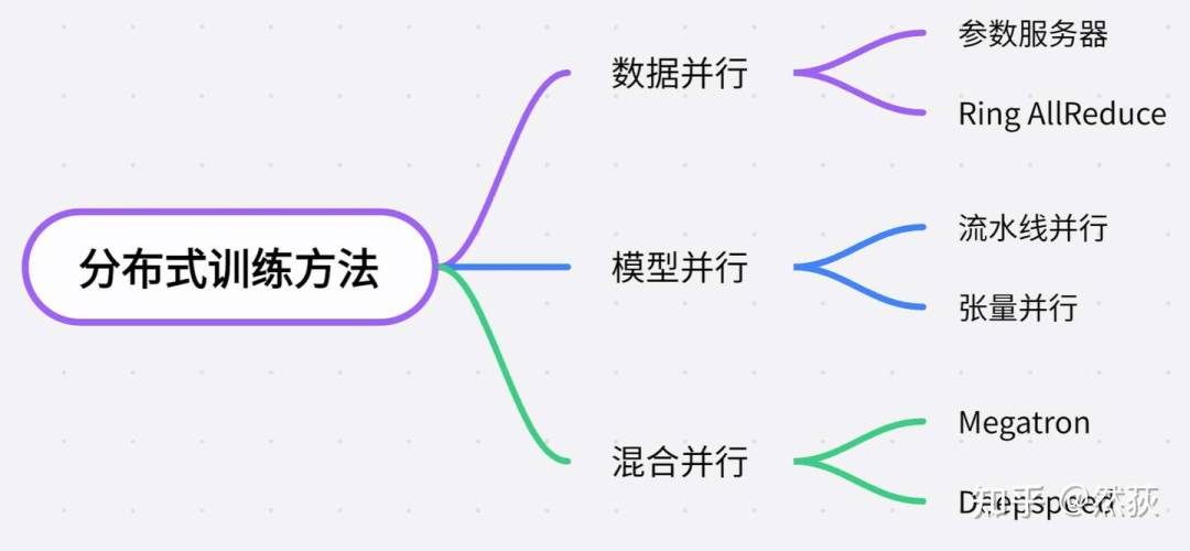
Based on the size of the model that needs to be loaded, distributed methods can generally be classified as follows:

• For small models that can be trained on a single card, distribution is mainly for training acceleration, typically using data parallelism, where each GPU has a copy of the model, and different data is fed to different GPUs for training.

• As models grow larger and cannot be trained on a single card, model parallelism is employed, which can be further divided into pipeline parallelism and tensor parallelism. Pipeline parallelism refers to splitting each layer of the model across different GPUs. When a model becomes so large that a single layer cannot be deployed on a single GPU, tensor parallelism is used to split the model layer for training.

• Deepspeed uses the Zero Redundancy Optimizer to further reduce memory usage during training, allowing for training larger models.

  

2. Necessary Knowledge Supplement

2.1 How Models Are Trained

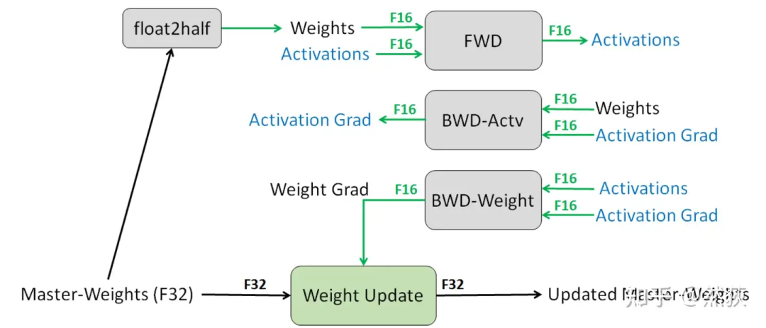
To understand how distributed training optimizes the model training process, it is essential to know how models are trained. Taking mixed precision training, which is currently the most widely used, as an example, the training process can be described as follows:

• Step 1: The optimizer first backs up a copy of the model weights in FP32 precision and initializes the first and second moment (used for updating weights).

• Step 2: Allocate a new storage space to convert the FP32 model weights into FP16 precision (used for forward and gradient computation).

• Step 3: Run forward and backward passes, storing the gradients and activation values in FP16 precision.

• Step 4: The optimizer uses the FP16 gradients and FP32 first and second moments to update the backed-up FP32 model weights.

• Step 5: Repeat Steps 2 to 4 until the model converges.

We can see that during training, memory is primarily consumed in four modules:

• Model weights (FP32 + FP16)

• Gradients (FP16)

• Optimizer (FP32)

• Activation values (FP16)

How to calculate the memory consumed during training? How large a model will exceed our maximum memory during training? For an analysis of memory usage during large model training, you can refer to the article “Understanding Memory Usage of Large Models (Single Card Consideration)” which is very detailed (self-promotion) and helpful for understanding how to optimize memory usage.

https://zhuanlan.zhihu.com/p/713256008

2.2 How GPUs Communicate

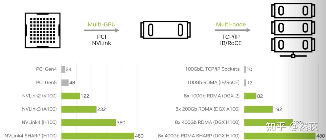
We often hear about single machine with 8 cards, multi-machine multi-card, and multi-node. Here, “single machine” and “node” refer to a single server, and 8 cards naturally refer to 8 GPUs. The 8 GPUs within the same server share the resources of the same host system (such as CPU resources, system memory, etc.). Different GPUs within the same node communicate via PCIe bus or NVLink (limited to NVIDIA cards), while GPUs between different nodes generally communicate via InfiniBand network cards (NVIDIA’s DGX system has one GPU card paired with one InfiniBand card). As shown below, the communication bandwidth between multiple nodes can reach a similar speed as that between multiple GPUs on a single node. You may wonder why NVLink is not used between nodes, because NVLink is designed for very short-distance communication, usually within the same server chassis, which is not convenient for expansion.

In addition to the hardware mentioned above, there is also software, namely the famous NCCL (NVIDIA Collective Communications Library), specifically designed for communication between multiple GPUs and even multiple nodes. AllReduce, Broadcast, Reduce, AllGather, and ReduceScatter are the main communication primitives implemented by NCCL.

In fact, NCCL provides an interface, and we do not need to understand how it is implemented at a low level; we just need to call the interface to achieve communication between GPUs.

2.2.1 Broadcast

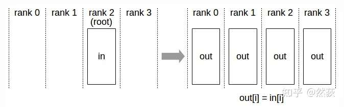
Broadcast refers to sending data from one GPU to all other GPUs simultaneously.

2.2.2 Scatter

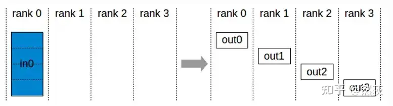
Scatter refers to splitting data from one GPU into multiple chunks and sending them sequentially to other GPUs.

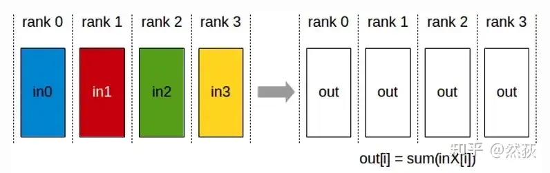
2.2.3 Reduce

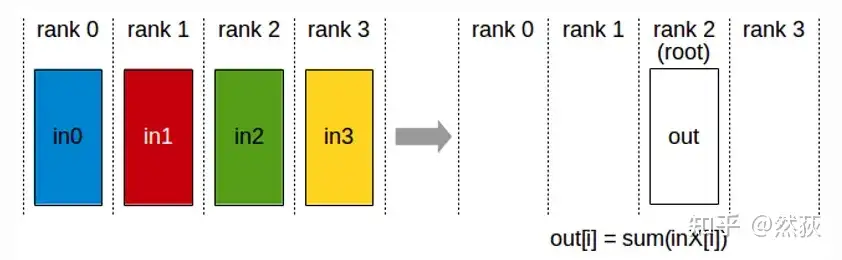
Reduce here serves to sum, i.e., sending data from multiple GPUs to a specified GPU and summing them.

2.2.4 Gather

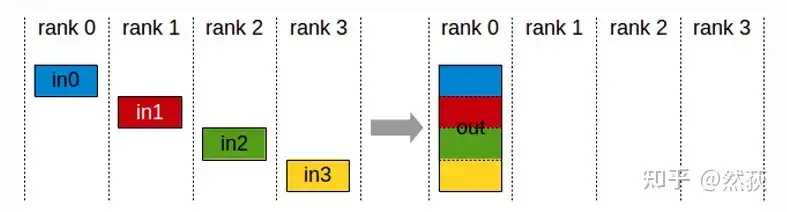
Gather is the reverse operation of Scatter, which merges data chunks scattered across different GPUs.

2.2.5 AllReduce

AllReduce means that each GPU sends data to the other GPUs, and each GPU sums the received data.

2.2.6 AllGather

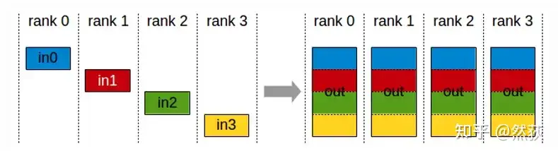
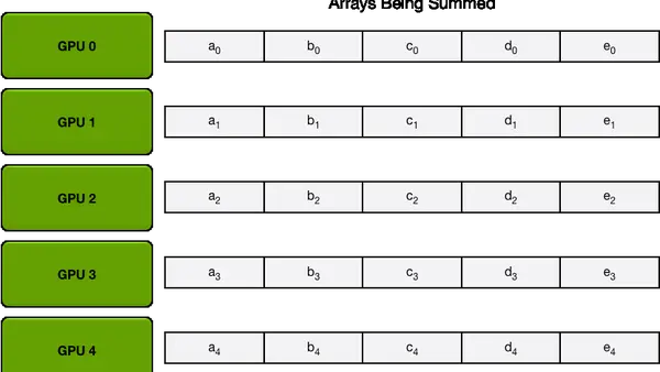
AllGather means that every GPU sends data to all other GPUs, and each GPU concatenates the received data into a complete dataset.

2.2.7 ReduceScatter

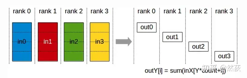
ReduceScatter means first performing Scatter and then Reduce, splitting the GPU data into multiple chunks, and then performing Scatter on each chunk according to the GPU sequence. After scattering all GPUs, the current GPU sums all the received data chunks, which is the Reduce operation.

If it seems confusing after reading, don’t worry; just have a general impression. You only need to know that these basic communication combinations between GPUs can achieve the various data transfers required for distributed systems.

3. Data Parallelism

Data parallelism refers to when the large model is initially small enough to fit comfortably on a single GPU. At this point, if we want to speed up training, besides increasing batch size, what else can we do? If one person is too slow at washing dishes, we can hire more people. Hiring more people means duplicating the model on multiple GPUs to get the job done.

3.1 Parameter Server

A very simple method is to select one of the eight monkeys as a supervisor, whose role is to collect the gradients from all the monkeys, then calculate the average gradient and send it back.

https://zhuanlan.zhihu.com/p/713256008

Here we introduce a concept of communication volume, which is used to measure the communication parameters of a single GPU or the entire system. We denote a complete set of parameters as Φ, which refers to a complete gradient parameter. Assuming there are N GPUs, the communication volume is as follows:

Does this method seem familiar? Yes, this is the previously mentioned ALL_Reduce method. This is also the method proposed by the parameter server in Li Mu’s paper. For more in-depth understanding, you can refer to the paper “Scaling Distributed Machine Learning with the Parameter Server”.

3.2 Ring AllReduce

Although the parameter server method is simple, it has two fatal flaws:

• (1) Too much redundancy: Each GPU has to copy a model weight, which leads to redundancy.

• (2) Unbalanced communication load: The server needs to communicate with every worker, while workers only need to send and receive once.

Ring AllReduce is a method used to solve the unbalanced load issue. We can understand the above method as a centralized method, while this method is decentralized, eliminating the distinction between server and worker, achieving balanced communication across all GPUs.

The entire process is actually the previously mentioned communication primitives of ReduceScatter followed by AllGather. For the communication volume calculation of Ring AllReduce, since it is a highly parallelized communication, we only need to consider the communication volume of a single GPU and then multiply by the number of GPUs for the total communication volume.

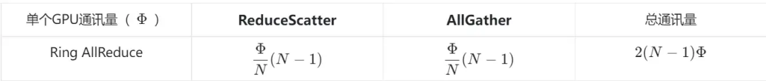
It is important to note that the total communication volume of the parameter server and Ring AllReduce is almost the same, but their communication times differ because the former has too high a communication load on the server side, causing delays and longer times. Currently, the commonly used DDP (Distributed Data Parallel) multi-machine multi-card training in Torch uses Ring AllReduce for communication.

4. Model Parallelism

The data parallelism mentioned above applies when the model is small enough to fit on a single GPU. However, in the era of large models, where models can have 70B parameters or more, a single card cannot accommodate them. What should we do? We can only disassemble the model. The fundamental difference between this distributed method and data parallelism is that the data in data parallelism is independent, while model parallelism involves splitting the model into parts that must use the same batch of data for processing.

4.1 Pipeline Parallelism

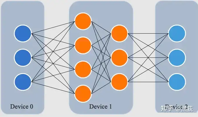
Pipeline parallelism refers to slicing the model layer by layer. Since the model is structured in layers, we can peel it off layer by layer.

4.1.1 Naive Pipeline

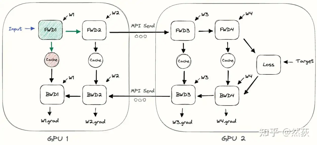
The naive pipeline is the simplest form of pipeline, where we sequentially perform forward passes layer by layer and then backward passes layer by layer. It is easy to understand. It is important to note that we pass the output tensor of the current layer between each layer, not the gradient information, thus the communication volume is relatively small. However, a smaller communication volume does not mean a higher overall utilization efficiency, as the parallelism between communication and computation and memory redundancy are also crucial factors to consider.

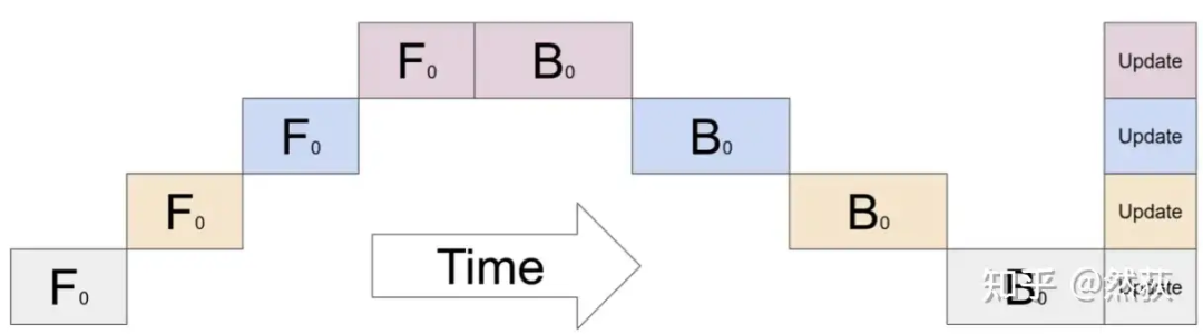
The image below shows a more concrete implementation of naive pipeline with two GPUs. We find that aside from the additional forward and backward information transfer in between, there is no difference in operation compared to running on a single GPU.

The naive pipeline is very simple, which leads to very obvious problems. We identify the two main issues:

1. Low GPU Utilization: As can be seen from our figure 4-2, all the blank spaces in the figure are wasted GPU space, referred to as bubbles. The bubble rate of the naive pipeline can be calculated as (Bubble Rate = (G – 1)/G), where G refers to the number of GPUs. It can be seen that the more GPUs there are, the closer the bubble rate approaches 1, which results in very low GPU utilization.

2. No Interleaving of Communication and Computation: When GPUs communicate between layers, all GPUs remain idle, and the communication and computation do not achieve a parallel mode, which significantly reduces training efficiency.

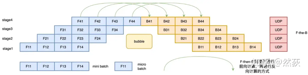
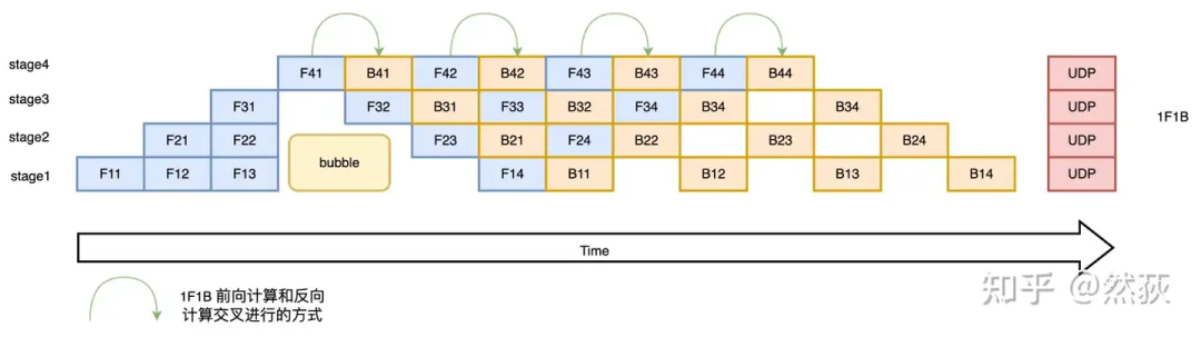
4.1.2 Micro-Batch Pipeline Parallelism

This method’s core idea is to use data parallelism to address the low GPU parallel efficiency of naive pipelines by splitting a large batch into multiple smaller batches for the pipeline. Let’s illustrate with a simple example: Zhang San and Li Si are processing a basket of fish using a naive pipeline, where Zhang San washes the fish, and Li Si cooks them. Li Si must wait for Zhang San to finish washing the entire basket before he can cook. Now they improve the process to micro-batch pipeline by dividing a large basket of fish into N smaller baskets. At this point, Zhang San can wash a small basket of fish and hand it to Li Si to cook, while Zhang San continues washing the next small basket, creating a parallel processing segment between them.

Now let’s look at the diagram below to understand this method, which is called the F-then-B mode pipeline strategy. In the micro-batch case, forward computation occurs first, followed by backward computation. The bubble rate of the F-then-B mode can be calculated as , where G is the number of GPUs and minibatch is the number of mini-batches. It can be seen that the bubble rate decreases significantly, and as the minibatch size increases, the effect becomes smaller.

What? You say it’s still not efficient enough? Then let’s look at the 1F1B (One Forward pass followed by One Backward pass) mode pipeline strategy, which is a method of interleaving forward and backward computations. In the 1F1B mode, forward and backward computations interleave, allowing for quicker release of unnecessary intermediate variables. As shown in the diagram, the green arrows indicate the distance between forward and backward computations; the distance is closer than in the F-then-B mode, which means this method can release unnecessary activation values more quickly after the backward pass. The bubble rate of the 1F1B mode can be calculated as . Hey, why does the bubble rate look exactly the same as in the F-then-B mode? Shouldn’t their efficiencies be the same? Why is it still considered optimized? This is because the interleaving of 1F1B mode allows for quick release of intermediate variables, which saves memory. Given a fixed device memory, we can increase the value (increase the number of micro-batches) to reduce the bubble rate.

4.2 Tensor Parallelism

While we discussed horizontal slicing for pipeline parallelism, vertical slicing refers to slicing based on the internal parameters (tensors) of each layer of the model.

From a mathematical perspective, tensor parallelism for linear layers involves block matrix multiplication, followed by merging the results; for non-linear layers, no additional design is required.

As shown in the diagram below, X is the input, A is the weight matrix, and Y is the output. We can slice the weight matrix A horizontally and vertically. The last two vectors of vertical slicing are merged, while the two vectors of horizontal slicing are summed, which is determined by the properties of matrix multiplication. This is the core principle of tensor parallelism; no matter how the methods are wrapped, they all revolve around these two matrix multiplication slices.

As mentioned earlier, tensor parallelism only occurs in linear layers. The diagram below illustrates the specific implementation of matrix multiplication for linear layers, including the specific computations and communications that occur during forward and backward passes.

5. Mixed Parallelism

In the previous sections, we introduced the basic implementation ideas of data parallelism and model parallelism. In this section, we will discuss how Megatron and DeepSpeed mix and optimize data parallelism and model parallelism in practical applications, achieving remarkable results. This article mainly focuses on the logical ideas to help you understand the overall picture without getting bogged down in the technical details, as discussing the details and depth of either Megatron or DeepSpeed alone would require extensive coverage.

5.1 Megatron

The core idea of Megatron is to combine model parallelism (MP), including tensor parallelism (TP) and pipeline parallelism (PP), with data parallelism (DP), also known as a 3D parallel strategy. Among these, tensor parallelism is the focus of Megatron, and it is the knowledge point we need to learn first. You might ask, didn’t we already discuss that tensor parallelism is based on horizontal or vertical slicing in linear layers? But do you know how to slice in the transformer architecture? When to slice horizontally and when to slice vertically? Which linear layers in the transformer can be sliced this way? These are the questions Megatron aims to answer first.

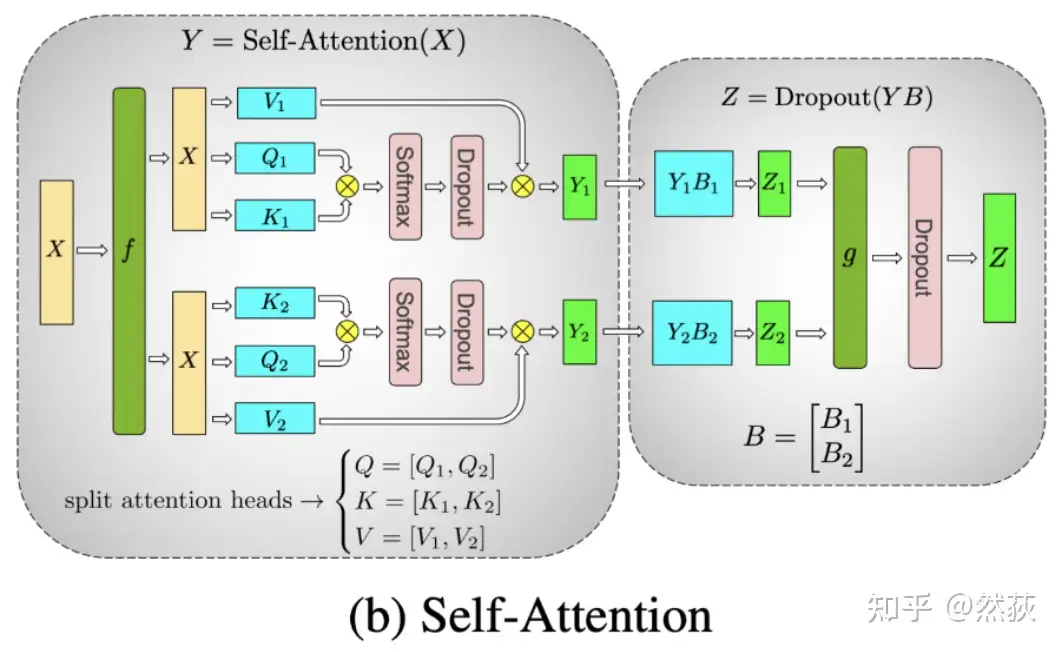
5.1.1 Review of Transformer Model Structure

I have drawn a simplified version of the transformer structure, aiming to highlight which parts contain linear layers. It clearly shows that we can divide the model into three sections: one for the input and output embedding layers, one for the multi-head attention layers, and one for the feedforward layers. Next, we will introduce how tensor parallelism is implemented for these three sections.

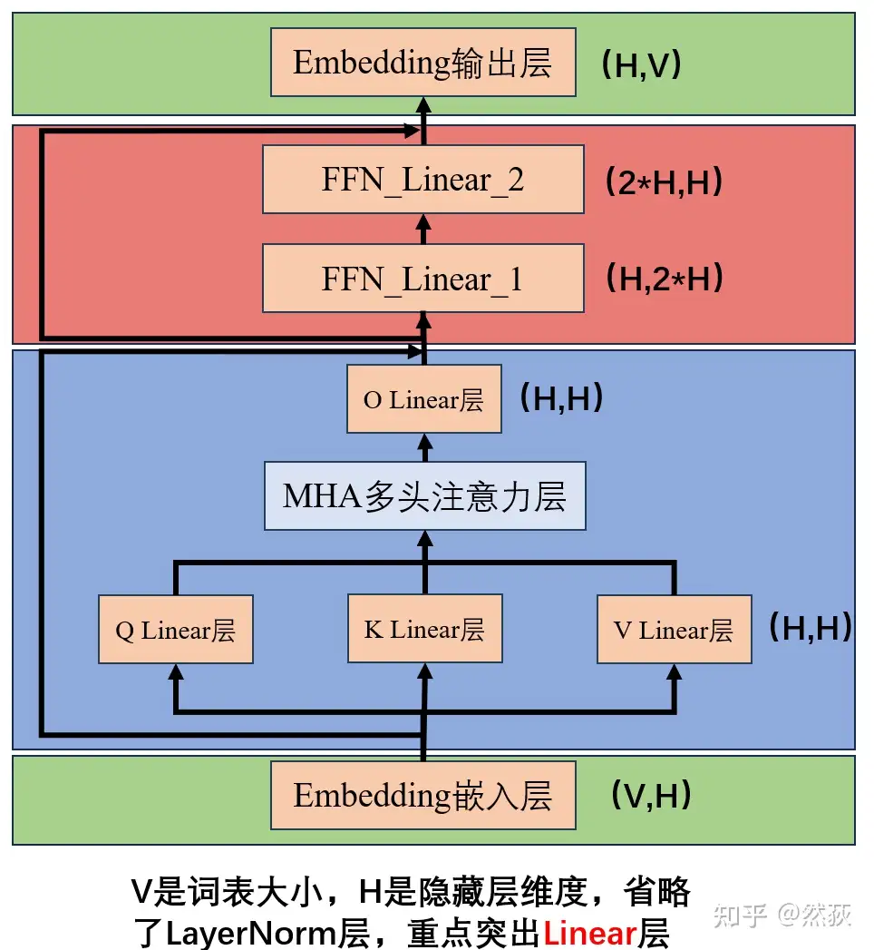
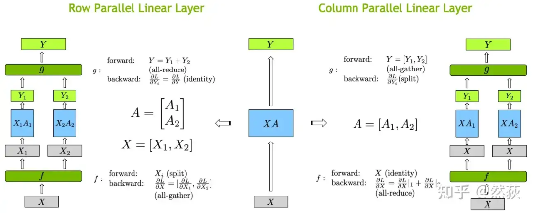
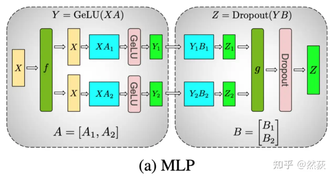
5.1.2 Tensor Parallelism in Feedforward Layers

We know that the feedforward layer consists of two linear layers, represented by weight matrices A and B in the diagram below. The tensor parallelism method here is quite simple and clear, where A is sliced vertically and B is sliced horizontally. Now, why is that?

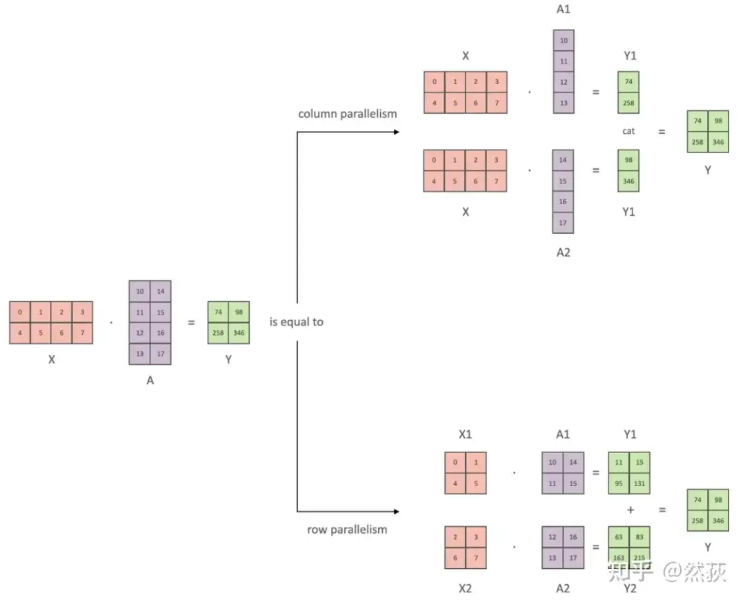
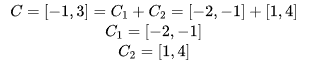
Let’s look at two equations: If

Where the colon represents concat

Which equation do you think is correct? I won’t keep you in suspense; the first addition equation is incorrect, while the second merging equation is correct.

Because Relu or any other arbitrary nonlinear function does not have properties similar to the distributive property of addition.

Let’s look at a simple example to clarify.

Relu (x) is just max (0, x).

It can be clearly seen that for non-linear activation functions, you cannot first separate and pass through the activation function before summing. The merging example is simpler, so I won’t elaborate.The results after passing through the activation function and merging are the same as merging first and then passing through the activation function.

We should also understand why the matrix is sliced vertically, as this way we avoid needing to communicate for addition before calculating the non-linear activation function; we only need to communicate once at the end to merge the results. After slicing the matrix vertically, due to the nature of matrix multiplication, the matrix can only be sliced horizontally.

Let’s analyze this in detail:

• Forward computation of f: Copy input X to two GPUs, allowing each GPU to perform forward computation independently.
• Forward computation of g: After completing the forward computation on each GPU, obtaining Z_1 and Z_2, the GPUs perform an AllReduce to sum the results to produce Z.
• Backward computation of g: We only need to copy the weights to two GPUs, allowing them to independently compute gradients.
• Backward computation of f: When the gradient for the current layer is computed and needs to be passed to the next layer, we need to obtain . At this point, the two GPUs perform an AllReduce to sum their respective gradients.

Thus, at this point, the two GPUs perform an AllReduce to sum their respective gradients.

5.1.3 Tensor Parallelism in Multi-Head Attention Layers

For multi-head attention, the method of tensor splitting is relatively unique. As shown in the diagram below, tensor parallelism is performed based on the number of heads, as each head can independently compute attention.

Specifically, we perform column slicing on the Q, K, V matrices and row slicing on the O matrix. This slicing method is similar to that of the FFN layer, aimed at reducing communication volume. The forward and backward computations are similar, involving two AllReduce operations, which I won’t elaborate further.

5.1.4 Tensor Parallelism in Embedding Layers

We know that for the embedding layer, the matrix dimensions are either (V,H) (input matrix) or (H,V) (output matrix).

The main reason for performing parallel splitting is that the V vocabulary dimension can easily exceed hundreds of thousands, while the H dimension (thousands of dimensions) is not even in the same order of magnitude. Thus, we only need to remember that for the embedding layer, we slice based on the V vocabulary dimension.

For the input embedding layer:

We will slice this dimension horizontally, resulting in each GPU having a weight dimension of

Similarly, we can conclude that for the output embedding layer, we will slice vertically, resulting in each GPU having a weight dimension of

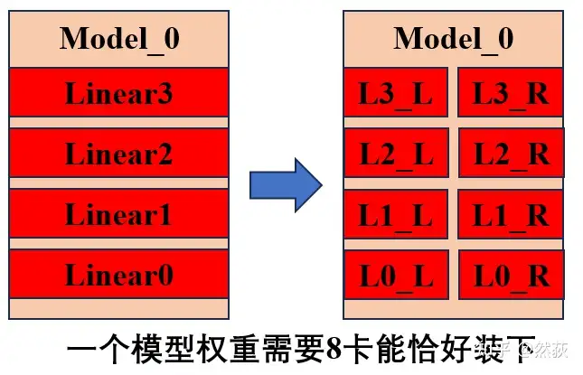
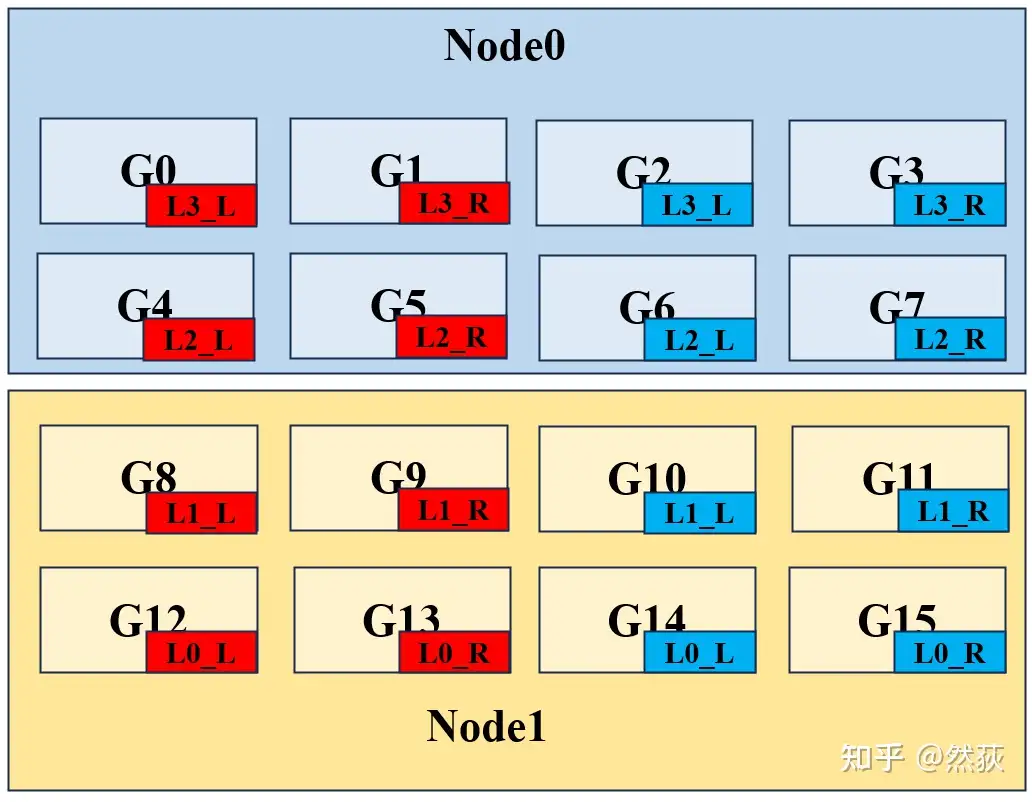
5.1.5 Example Analysis of 3D Parallelism

Here I will provide an example to help everyone understand how Megatron’s 3D parallelism is specifically applied.

Suppose we have two machines, each with 8 GPUs, and our model requires 8 GPUs to fit completely, consisting of 4 linear layers.

First, we will use pipeline parallelism to split the model into four layers, but we find that even one layer cannot fit on a single GPU, so we will apply tensor parallelism to split the weights of each layer in half. At this point, we split a model into eight parts, each of which can fit onto a GPU.

Generally, the ranking of communication volume is: TP (tensor parallelism) > DP (data parallelism) > PP (pipeline parallelism). To minimize communication volume, the larger parts should ideally be kept within a single machine, as the bandwidth within a node is higher than between nodes. Based on this consideration, we perform the following segmentation.

As shown in the diagram below, the red and blue represent two independent complete models split into eight parts. L and R correspond to the tensor splitting mode of a linear layer. It can be seen that all paired L and R tensor parallelism are placed within the same node to prioritize ensuring communication for tensor parallelism. Then, we consider data parallelism and pipeline parallelism, placing layers 0 and 1, and layers 2 and 3 on different nodes, as the communication volume for pipeline parallelism is relatively low.

5.2 DeepSpeed

To fully understand DeepSpeed, please review the previously mentioned model training process and memory usage (section 2.1 summary) as well as GPU communication primitives (section 2.2 summary) for a deeper understanding.

Assuming we have a GPU with infinite memory, there would be no need for data parallelism (here you can think about why model parallelism is necessary even with an infinitely large GPU). In other words, our data parallelism fundamentally relies on communication to exchange for memory. DeepSpeed’s famous Zero mechanism is based on this idea.

Some students who have learned about the Zero mechanism might think its method resembles model parallelism since it involves splitting optimizer parameters, model weights, and gradients. However, the Zero mechanism is indeed a form of data parallelism because during forward and backward passes, a complete model weight is still required.

The essence of model parallelism is to split a large model weight into smaller parts, each of which can run independently on a single GPU; data parallelism requires a complete model weight (which can be an entire model or a split layer model, as long as the model is independent) to run on a single GPU, while we simply want to fit more data. Although the Zero mechanism involves many splits, it still requires complete model weights during forward and backward passes. If you don’t understand it now, that’s okay; keep reading, and it will gradually make sense.

Let’s briefly review the steps of model training:

1. Model weights perform forward and backward passes to obtain gradients.
2. Use gradients to update the first and second moments of the optimizer (Adam).
3. Update model weights using the optimizer.

The following image used to confuse me a lot, where the contents in each blue box are what I thought were necessary memory for the current step.

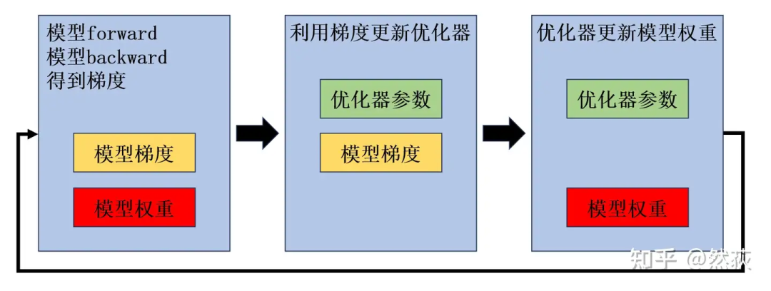
• In the first image: During the backward pass, memory will certainly contain model weights and gradients, but optimizer parameters are not needed.
• In the second image: When updating the first and second moments of the optimizer, model weights are not required.
• In the third image: When using the optimizer’s first and second moments to update model weights, gradients should not be needed anymore and can be released.

However, the actual situation is that model weights, gradients, and optimizer parameters continuously occupy memory.

1. The significance of the first and second moment parameters of the optimizer is to store historical gradient information and changes, so they cannot be released and must occupy memory waiting to be updated.
2. Model weights are the parameters we need to update, so they must always be stored in memory waiting for updates.
3. Gradients are different each time; can they be released? Actually, no, because the second and third steps are combined, which means that the optimizer.step() function requires the gradients to be retained until the weights are updated, but then it enters the next forward and backward passes, and the gradients remain stored (I actually find this strange; I wonder if anyone can clarify this, as I feel the gradients could theoretically be released).

In summary, during actual training, many redundant parameters occupy memory, even when they are not needed at the current stage. How should we optimize these redundancies? The answer is to slice and distribute. By slicing, we exchange communication for memory, transferring data when needed and releasing it when not.

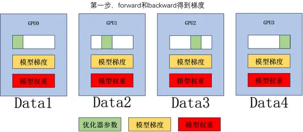
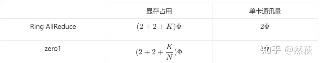
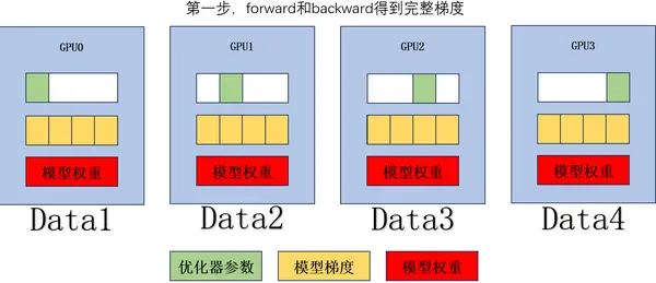
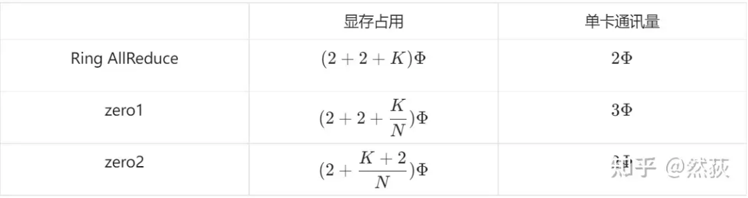
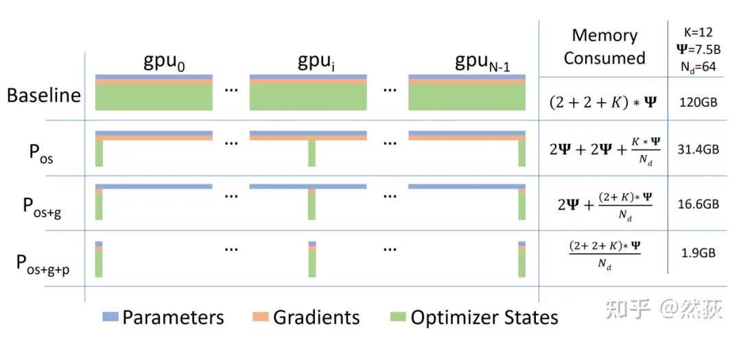
5.2.1 Zero1: Slicing Optimizer States

We will compare this to Ring AllReduce, excluding model parallelism for clearer understanding of Zero’s approach.

Assuming that the model has parameters , the total number of GPUs is , the memory for model weights is , the memory for model gradients is , and the memory for the optimizer is (since different optimizers can have different memory usage, Adam consumes a lot, which is why we prioritize slicing the optimizer).

Let’s understand how training works after slicing the optimizer using the following steps and animations:

1. Perform forward and backward passes to obtain gradients.
2. Perform Ring AllReduce on the gradients to obtain the average gradient, with a single GPU communication volume of .
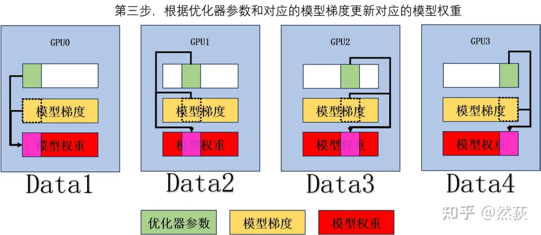
3. Update the corresponding model weights based on the optimizer parameters and corresponding model gradients.
4. Perform AllGather on the updated model weights, with a single GPU communication volume of .



Finally, let’s summarize the memory and communication volume in the table below. It is easy to understand that the memory for the optimizer part is divided by , distributed across all GPUs, and the single GPU communication volume can be derived from our previous analysis to increase to .



Those who are attentive may notice that during this phase, we only use a portion of the model gradients on each GPU, which is the part in the dashed box, while the rest is redundant. This is actually the point that Zero2 will optimize: splitting the gradients.

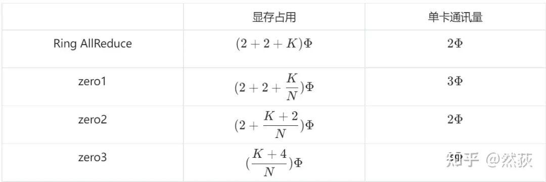
5.2.2 Zero2: Slicing Gradients

Let’s directly look at the steps and animations; you can gradually understand them in conjunction with the previous communication primitives, which are quite interesting:

1. Perform forward and backward passes to obtain complete gradients.
2. Perform ReduceScatter on the gradients, with a single GPU communication volume of .
3. Update the corresponding model weights based on partial gradients and corresponding optimizer parameters.
4. Perform AllGather on the model weights, with a single GPU communication volume of .



Let’s also add the memory and communication volume table:



Some may notice that during the first step, we obtained complete gradients before ReduceScatter. Shouldn’t the memory be at this point? Shouldn’t the memory limit still be this much? I believe we utilized CPU memory as a temporary buffer, which is about to be replaced by the gradients from ReduceScatter. In the later stages, we can see that after AllGather, the model will have a temporary buffer to store the results.

Interestingly, Zero2 uses the same communication volume as Ring AllReduce but significantly reduces memory usage, which is the so-called redundancy reduction effect.

5.2.3 Zero3: Slicing Model Weights

I initially wanted to create a GIF to demonstrate this, but I encountered some confusion while drawing, and I found the official demonstration video below, which is incredibly clear. If you carefully understand the previous content, this video will be very easy to comprehend. It’s a fantastic video.

My personal recommendation is to watch it; I previously read many blogs but didn’t understand much until I watched this video. Thinking about it, it’s indeed difficult to describe this dynamic implementation without ambiguity in language. Trust me, watching this video is definitely faster than slowly deciphering those blogs.

To summarize:

From the overall process, model weights undergo two AllGather operations, while gradients perform one ReduceScatter. However, these AllGather and ReduceScatter operations differ from previous ones; they interleave with the entire process of forward and backward passes, which is something you must carefully appreciate in conjunction with the video for clarity.

Finally, we have obtained this comprehensive summary image from the paper “ZeRO: Memory Optimizations Toward Training Trillion Parameter Models”. Does everything seem clearer now?

6. Summary

I initially only wanted to outline the logic of the entire technical chain, but I ended up writing so much content that it exhausted me. I feel there’s not much to summarize, so I’ll leave it at that for now. Any gaps or issues will be supplemented later. After all, it’s best to produce a rough draft first and then revise it gradually.

Technical Communication Group Invitation

△ Long press to add assistant

Scan the QR code to add the assistant on WeChat

Please note: Name – School/Company – Research Direction

(e.g., Xiaozhang – Harbin Institute of Technology – Dialogue Systems)

to apply to join technical communication groups like Natural Language Processing/PyTorch

About Us

MLNLP community is a grassroots academic community built by scholars in machine learning and natural language processing both domestically and internationally. It has developed into a well-known community for machine learning and natural language processing, aiming to promote progress among academic and industrial circles in machine learning and natural language processing, as well as among enthusiasts.

The community can provide an open communication platform for related practitioners in further education, employment, and research. Everyone is welcome to follow and join us.