Source: Algorithm Advancement

This article is about 2000 words long and is recommended to be read in 8 minutes. This article uses illustrations to help everyone quickly understand the principles of Diffusion.
[ Introduction ]Many of you have probably heard about the deep generative model Diffusion Model that is gaining popularity in the field of images. To help everyone quickly understand the principles of Diffusion, this article presents it in a visual manner. I hope this helps you advance in your learning and application of AIGC technology!
1. Diffusion Text-to-Image Generation – Overall Structure
1.1 The Entire Generation Process
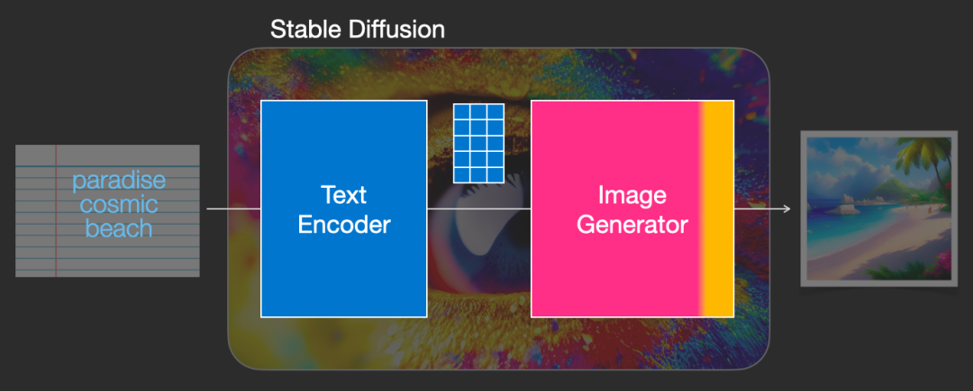
We know that when using Diffusion, images are generated from text. However, in the previous article, the input to the Diffusion model was only random Gaussian noise and time step. So how does text get converted into Diffusion’s input? What changes when text is added? The answer can be found in the diagram below.
▲ The entire process of generating images from text
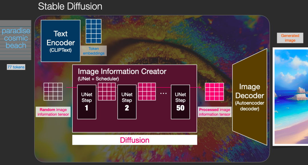
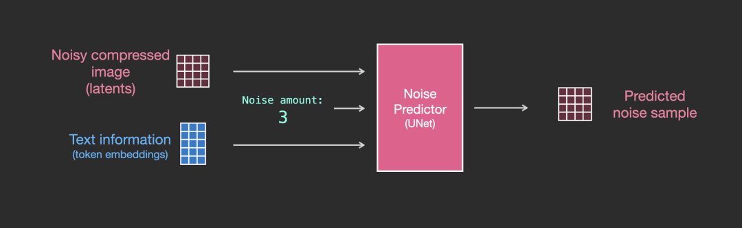
In fact, Diffusion uses a Text Encoder to generate the corresponding embedding for the text (the Text Encoder uses the CLIP model), which, together with the random noise embedding and time step embedding, serves as the input for the Diffusion model to ultimately generate the desired image. Let’s take a look at the complete diagram:
▲ Token embedding, random noise embedding, and time embedding are input into diffusion together
From the above diagram, we see that the input to Diffusion consists of token embeddings and random embeddings, while the time embedding is not shown. The Image Information Creator in the middle consists of multiple UNet models, and a more detailed diagram is shown below:
▲ More detailed structure
We can see that the Image Information Creator in the middle is composed of multiple UNets. We will discuss the structure of UNet later. Now that we understand the structure of Diffusion after adding text embeddings, how are the text embeddings generated? Next, we will introduce how to use the CLIP model to generate text embeddings.
1.2 Generating Input Text Embeddings Using the CLIP Model
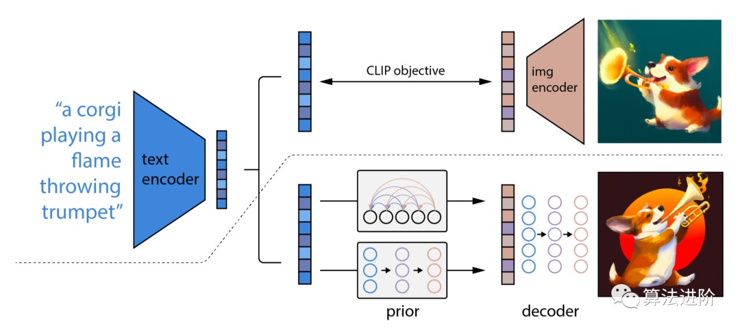
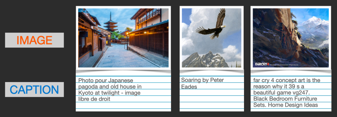
CLIP is trained on datasets of images and their descriptions. Imagine a dataset that looks like this, containing 400 million images and their descriptions:
▲ Images and their textual descriptions
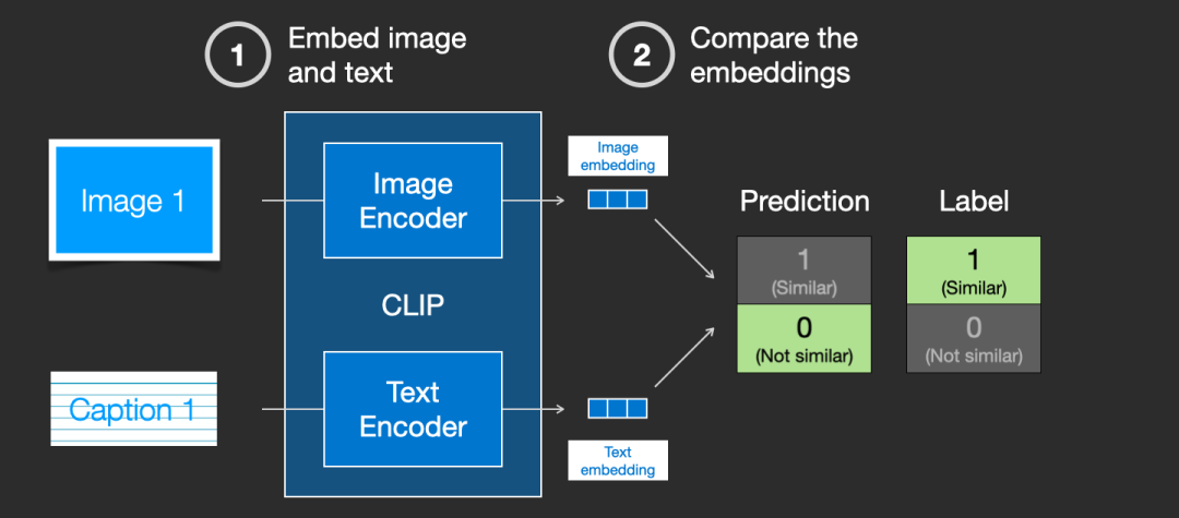
In fact, CLIP is trained based on images and their textual descriptions scraped from the internet. CLIP is a combination of an image encoder and a text encoder, and its training process can be simplified to adding textual descriptions to images. First, the image and text are encoded separately using their respective encoders.
Then, cosine similarity is used to characterize whether they match. Initially, the similarity will be very low.
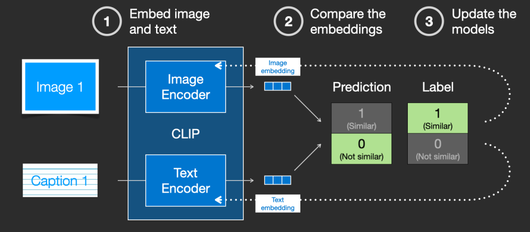
Then the loss is computed, and the model parameters are updated to obtain new image embeddings and text embeddings.
By training the model on the training set, we ultimately obtain the text embeddings and image embeddings. For details about the CLIP model, you can refer to the corresponding paper:
https://arxiv.org/pdf/2103.00020.pdf
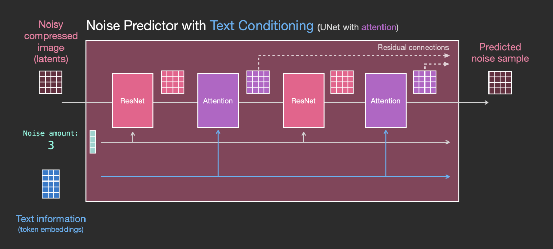
1.3 How Text Embeddings Are Used in the UNet Network
We have already introduced how to generate input text embeddings. So how does the UNet network use them? In fact, an Attention mechanism is added between each ResNet in the UNet, with one end of the Attention taking the text embeddings as input. The diagram below illustrates this:
A more detailed diagram is shown below:
Having introduced how Diffusion generates images from input text, we will now provide a detailed explanation of how the Diffusion model is trained and how it generates images.
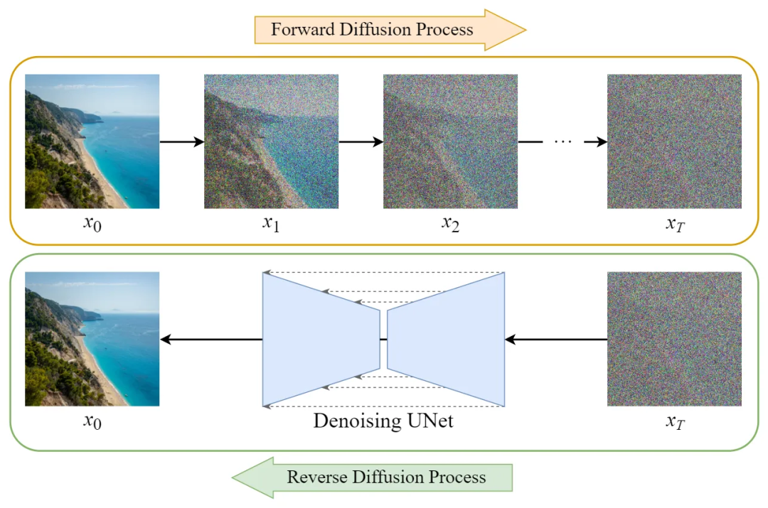
2.1 Training Process of the Diffusion Model
The training of the Diffusion model can be divided into two parts:
1. Forward Diffusion Process → adding noise to the image;
2. Reverse Diffusion Process → removing noise from the image.
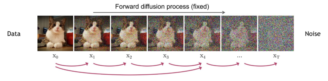
2.2 Forward Diffusion Process
The forward diffusion process involves continuously adding Gaussian noise to the input image.
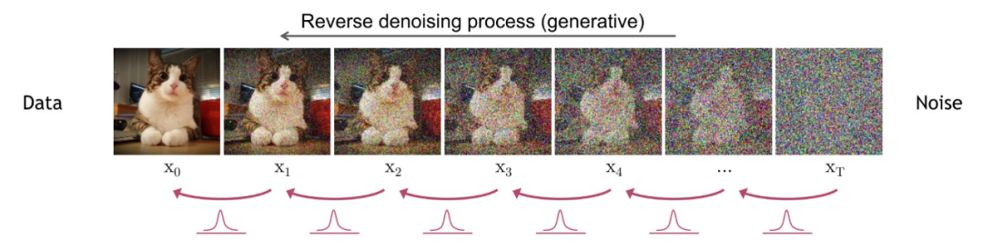
2.3 Reverse Diffusion Process
The reverse diffusion process involves continuously restoring the noise to the original image.
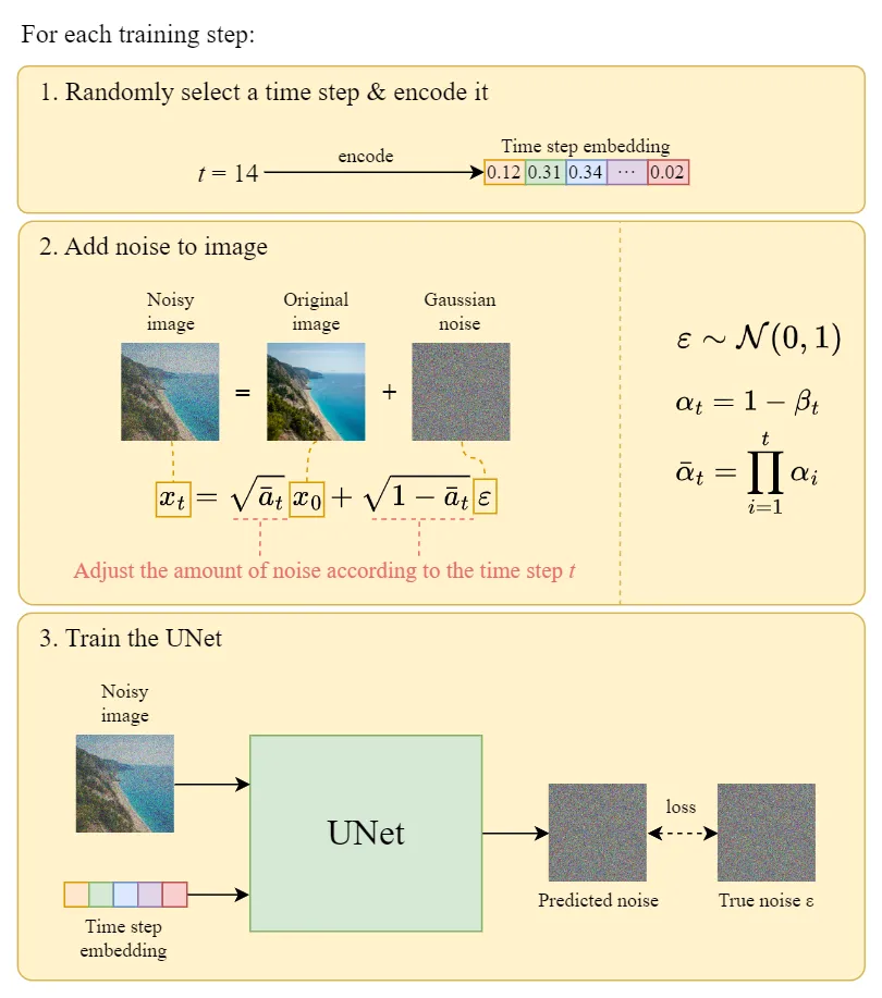
Each round of training includes the following steps:
1. For each training sample, a random time step t is chosen.
2. The Gaussian noise corresponding to time step t is applied to the image.
3. The time step is converted into the corresponding embedding.
Below is a detailed training process for each round:
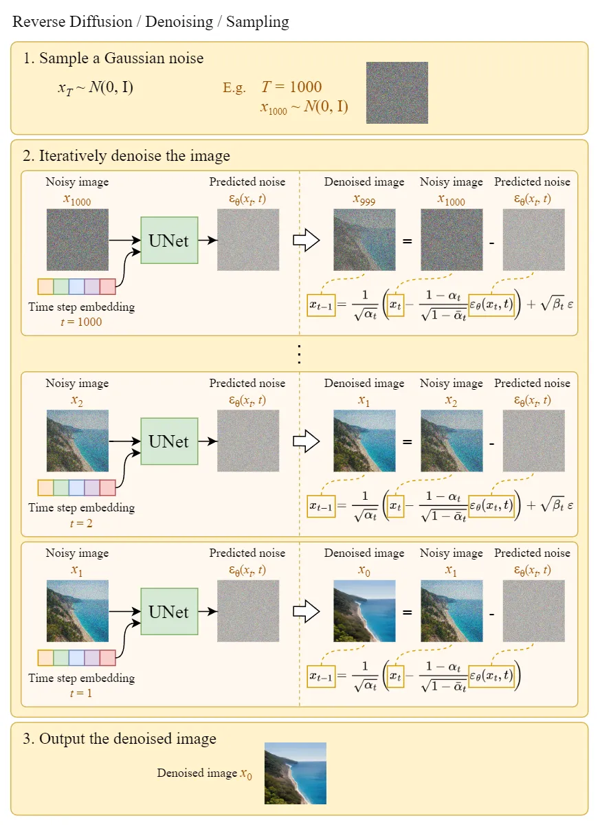
2.5 Generating Original Images from Gaussian Noise (Reverse Diffusion Process)
The “Sample a Gaussian” in the image indicates generating random Gaussian noise, while “Iteratively denoise the image” indicates the reverse diffusion process, which shows how to gradually transform Gaussian noise into the output image. It can be seen that the final generated Denoised image is very clear.
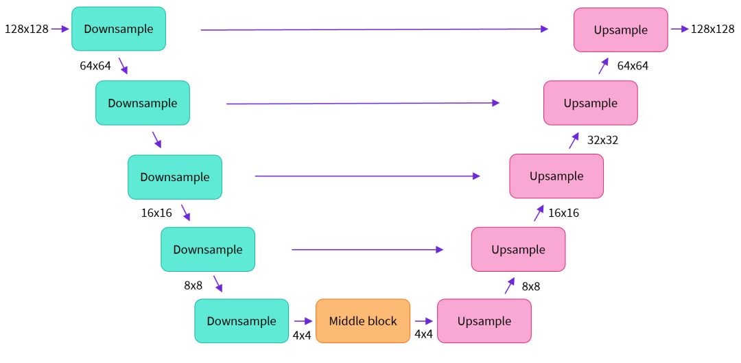
Supplement 1: UNet Model Structure
Having introduced the entire process of Diffusion, here is a supplement about the structure of the UNet model, as shown in the diagram below.
Inside, Downsample, Middle block, and Upsample all contain ResNet residual networks.
Supplement 2: Disadvantages of the Diffusion Model and Improved Version – Stable Diffusion
Previously, we used Stable Diffusion in the architecture of generating images from text. In fact, Stable Diffusion is an improved version of Diffusion.
The disadvantage of Diffusion is that during the reverse diffusion process, the entire size of the image must be input into the U-Net, which makes Diffusion very slow when the image size and time step t are sufficiently large. Stable Diffusion was proposed to solve this problem. We will discuss how Stable Diffusion improves upon this later.
Supplement 3: UNet Network Inputting Text Embeddings Simultaneously
In Section 2, when introducing the principles of Diffusion, for convenience, we did not include the input text embeddings, only using time embeddings and random Gaussian noise. For information on how to include text embeddings, please refer to Section 1.3.
Supplement 4: Why Introduce Time Step t in DDPM
The introduction of the time step t is to simulate a disturbance process that gradually increases over time. Each time step t represents a disturbance process that gradually changes the distribution of the image by applying noise multiple times from the initial state. Therefore, smaller t represents weaker noise disturbances, while larger t represents stronger noise disturbances.
There is another reason: in DDPM, all UNets share parameters. How to generate different outputs from different inputs, and ultimately transform a completely random noise into a meaningful image, is still a very difficult problem. We hope that during the initial reverse process, this UNet model can first generate some rough outlines of objects, and as the diffusion model progresses, it can learn high-frequency feature information when generating realistic images. Since all UNets share parameters, we need time embedding to remind the model of our current step, whether we want the output to be rough or detailed.
Thus, the introduction of time step t helps both the generation and sampling processes.
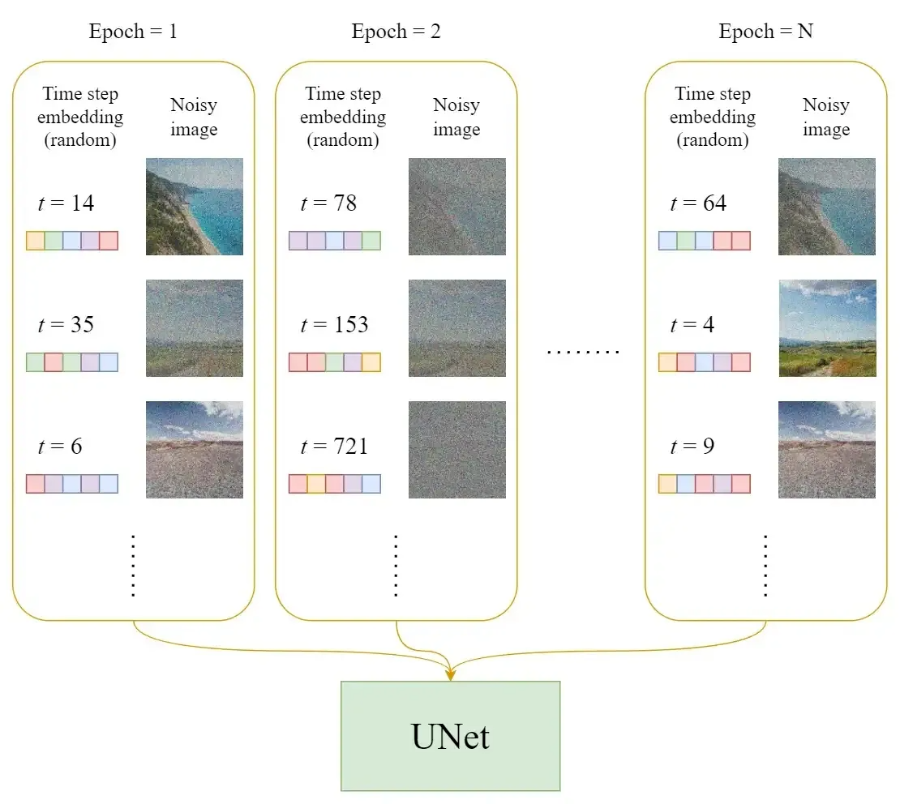
Supplement 5: Why Introduce Random Time Step t in Each Training Process
We know that the model’s loss gradually decreases during training, and the change in loss becomes smaller towards the end. If the time step is incremental, it will cause the model to focus too much on the earlier time steps (because the early loss is larger) and neglect the information from later time steps.
© Author | Confidential Ambush
Unit | Senior Algorithm Expert at Qihoo 360
https://medium.com/@steinsfu/stable-diffusion-clearly-explained-ed008044e07e
http://jalammar.github.io/illustrated-stable-diffusion/
https://pub.towardsai.net/getting-started-with-stable-diffusion-f343639e4931
https://zhuanlan.zhihu.com/p/597924053
https://zhuanlan.zhihu.com/p/590840909?
https://arxiv.org/abs/2103.00020
Editor: Huang Jiyan
Proofreader: Lin Yilin