
Click on the above“Beginner Learning Vision” and choose to add Star or Pin.
Important content delivered in real-time.Introduction
For almost all machine learning algorithms, whether supervised learning, unsupervised learning, or reinforcement learning, it generally boils down to solving an optimization problem. Therefore, optimization methods occupy a central position in the derivation and implementation of machine learning algorithms. In this article, the author will provide a comprehensive summary of the optimization algorithms used in machine learning and clarify their direct relationships, helping you understand this part of knowledge from a global perspective.
Mathematical Models Required by Machine Learning
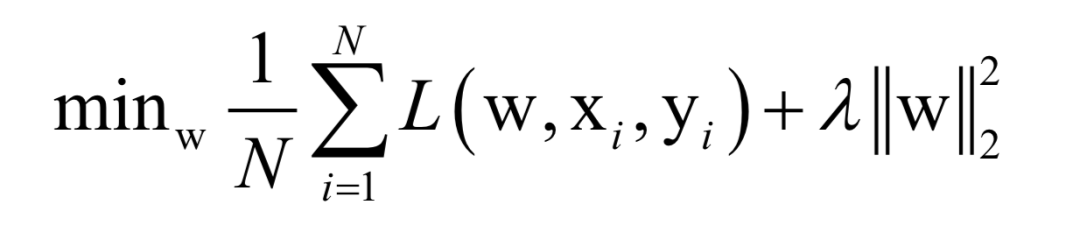
Almost all machine learning algorithms ultimately reduce to finding the extreme value of an objective function, i.e., an optimization problem. For example, in supervised learning, we want to find the best mapping function f(x) that minimizes the loss function for training samples (minimizing empirical risk or structural risk):

Here, N is the number of training samples, L is the loss function for a single sample, w is the model parameters to be solved, which are parameters of the mapping function, xi is the feature vector of the sample, and yi is the label value of the sample.
Alternatively, we may find an optimal probability density function p(x) that maximizes the log-likelihood function for training samples (maximum likelihood estimation):

Here, θ is the model parameters to be solved, which are parameters of the probability density function.
For unsupervised learning, taking clustering algorithms as an example, the algorithm aims to minimize the sum of distances of each class’s samples to the class center:

Here, k is the number of types, x is the sample vector, μi is the class center vector, and Si is the sample set of the ith class.
For reinforcement learning, we need to find an optimal policy, which is a mapping function from state s to action a (deterministic policy; for stochastic policy, it is the probability of executing each action):

So that for any given state, after executing the action a determined by this policy function, the cumulative reward is maximized:

Here, the state value function is used.
Overall, the core goal of machine learning is to provide a model (usually a mapping function) and then define an evaluation function (objective function) to evaluate the quality of this model, solving for the maximum or minimum of the objective function to determine the model parameters, thus obtaining the desired model. Among these three key steps, the first two are the problems that machine learning needs to study, establishing mathematical models. The third problem is a pure mathematical one, namely optimization methods, which is the core of this article.
Classification of Optimization Algorithms
For the various optimization objective functions of machine learning algorithms with different forms and characteristics, we have found various solving algorithms suitable for them. Except for a few problems that can be solved by brute force search to obtain the optimal solution, we divide the optimization algorithms used in machine learning into two types (this article does not consider stochastic optimization algorithms such as simulated annealing, genetic algorithms, etc.):
-
Analytical Solutions
-
Numerical Optimization
The former provides an exact analytical solution to an optimization problem, generally a theoretical result. The latter is used when it is very difficult to provide an exact calculation formula for the extreme point, using numerical methods to approximate the optimal point. In addition, there are other solving ideas, such as divide-and-conquer, dynamic programming, etc. A good optimization algorithm needs to meet:
-
Can correctly find extreme points in various situations
-
Fast speed
The following diagram shows the classification of these algorithms and their relationships:

Next, we will explain according to this diagram.
Fermat’s Theorem
For a differentiable function, the unified approach to finding its extreme value is to look for points where the derivative is 0, which is Fermat’s theorem. This theorem in calculus states that for a differentiable function, the derivative must be 0 at extreme points:

For multivariable functions, the gradient must be 0:

Points where the derivative is 0 are called stationary points. It is important to note that a derivative of 0 is only a necessary condition for the function to obtain extreme values, not a sufficient condition; it is merely a suspected extreme point. Whether it is an extreme value, whether it is a maximum or minimum, still needs to look at higher-order derivatives. For univariate functions, assuming x is a stationary point:
-
If f”(x) > 0, then there is a minimum at that point
-
If f”(x) < 0, then there is a maximum at that point
-
If f”(x) >= 0, we need to look at higher-order derivatives
For multivariable functions, assuming x is a stationary point:
-
If the Hessian matrix is positive definite, the function has a minimum at that point
-
If the Hessian matrix is negative definite, the function has a maximum at that point
-
If the Hessian matrix is indefinite, we need to look at higher orders (this part is incorrect)
At points where the derivative is 0, the function may not take extreme values, which is called a saddle point. The following diagram is an example of a saddle point (from SIGAI Cloud Laboratory):

In addition to saddle points, optimization algorithms may also encounter another problem: the local extreme value problem, where a stationary point is an extreme point but not a global extreme point. If we impose constraints on the optimization problem, we can effectively avoid these two problems. A typical case is convex optimization, which requires that the feasible region of the optimization variables is a convex set, and the objective function is a convex function.
Although stationary points are only a necessary condition for the function to achieve extreme values, it is much easier to find and filter whether they are extreme points once we have found stationary points. Whether in theoretical results or numerical optimization algorithms, finding stationary points is generally the goal of finding extreme points. For univariate functions, we first differentiate, then solve the equation of the derivative equal to 0 to find all stationary points. For multivariable functions, we take partial derivatives of each variable, set them to 0, and solve the system of equations to achieve all stationary points. These are basic methods taught in calculus. Fortunately, in machine learning, many objective functions are differentiable, so we can use this set of methods.
Lagrange Multiplier Method
Fermat’s theorem provides the necessary condition for the extreme value of a function without constraints. For some practical application problems, there are generally equality or inequality constraints. For optimization problems with equality constraints, the classic solution is the Lagrange multiplier method.
For the following problem:

Construct the Lagrange multiplier function:

At the optimal point, the derivatives with respect to x and the multiplier variables λi must both be 0:

Solving this equation will yield the optimal solution. For a more detailed explanation of the Lagrange multiplier method, you can read any advanced mathematics textbook. The places where the Lagrange multiplier method is used in machine learning include:
-
Principal Component Analysis
-
Linear Discriminant Analysis
-
Laplacian Eigenmaps in Manifold Learning
-
Hidden Markov Models
KKT Conditions
KKT conditions are a generalization of the Lagrange multiplier method, used to solve functions with both equality and inequality constraints. For the following optimization problem:

Similar to the Lagrange dual approach, the KKT conditions construct the following multiplier function:

λ and μ are called KKT multipliers. At the optimal solution x*, the following conditions should be met:

The equality constraint hj(x*) = 0 and the inequality constraint gk(x*) <= 0 are constraints that must be satisfied. ▽xL(x*) = 0 is similar to the previous Lagrange multiplier method. The only additional condition is regarding gi(x):

KKT conditions are only necessary conditions for achieving extreme values, not sufficient conditions. In machine learning, KKT conditions are used in:
-
Support Vector Machines (SVM)
Numerical Optimization Algorithms
The three methods discussed earlier can be used in theoretical derivation or in cases where root-finding formulas for certain equations (such as linear functions, maximum likelihood estimation of normal distributions) can be obtained. However, for the vast majority of functions, the equations where the gradient equals 0 cannot be solved directly, such as when the equations contain transcendental functions like exponential functions or logarithmic functions. For such unsolvable equations, we can only use approximate algorithms to solve them, which are numerical optimization algorithms. These numerical optimization algorithms generally utilize the derivative information of the objective function, such as first-order and second-order derivatives. If the first-order derivative is used, it is called a first-order optimization algorithm. If the second-order derivative is used, it is called a second-order optimization algorithm.
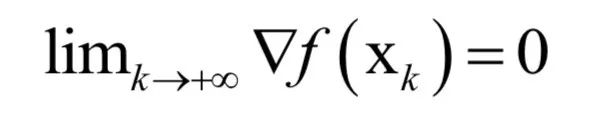
In engineering implementation, iterative methods are usually adopted, starting from an initial point x0, repeatedly moving from xk to the next point xk+1 according to certain rules, constructing such a sequence until converging to the point where the gradient is 0. That is, the following limit holds:
These rules generally utilize first-order derivative information, i.e., the gradient; or second-order derivative information, i.e., the Hessian matrix. Thus, the core of the iterative method is to obtain an iterative formula determined by the previous point to determine the next point:

Gradient Descent Method
The gradient descent method searches in the opposite direction of the gradient, utilizing the first-order derivative information of the function. The iterative formula for the gradient descent method is:
According to the first-order Taylor expansion of the function, in the negative gradient direction, the function value decreases. As long as the learning rate is set small enough and does not reach the point where the gradient is 0, the function value will definitely decrease with each iteration. The reason for setting the learning rate to a very small positive number is to ensure that the value xk+1 after iteration is within the neighborhood of the previous value xk, thus allowing us to ignore the higher-order terms in the Taylor expansion and ensure that the function value decreases during iteration.
The gradient descent method and its variants are widely used in machine learning, especially in deep learning. (Further reading: An Overview of Neural Network Optimization Algorithms)
Momentum Term
To accelerate the convergence speed of the gradient descent method and reduce oscillation, a momentum term is introduced. The parameter update formula with this term added is:

Where Vt+1 is the momentum term, which replaces the previous gradient term. The calculation formula for the momentum term is:

It is a weighted average of the previous momentum term and the current gradient value, where α is the learning rate and μ is the momentum term coefficient. If we expand according to time t, then in the t-th iteration, all gradient values from the first to the t-th iteration are used, and the old gradient values decay exponentially with coefficient μt:

The momentum term accumulates the gradient values from previous iterations, allowing this iteration to move forward in the direction of previous inertia.
AdaGrad Algorithm
AdaGrad is the most direct improvement to the gradient descent method. The gradient descent method relies on a manually set learning rate, which if set too small, converges too slowly, and if set too large, may cause the algorithm not to converge; setting an appropriate value for the learning rate is very difficult.
AdaGrad dynamically adjusts the learning rate based on the historical gradient values from previous iterations, and each component of the optimization variable vector X has its own learning rate. The parameter update formula is:

Where α is the learning factor, gt is the gradient vector of the parameters at the t-th iteration, and ε is a very small positive number to avoid division by 0. The only difference from standard gradient descent is the term in the denominator, which accumulates the historical gradient values up to this iteration to generate the coefficients for gradient descent. According to this formula, the absolute value of the historical derivative value determines the learning rate; the larger the historical gradient value, the smaller the component learning rate, and vice versa. Although it achieves adaptive learning rates, this algorithm still has problems: it requires a manually set global learning rate α, and as time accumulates, the denominator in the formula grows larger, leading to the learning rate approaching 0 and the parameters becoming unable to update effectively.
RMSProp Algorithm
RMSProp is an improvement to AdaGrad that avoids the problem of the learning rate approaching 0 due to the long-term accumulation of gradient values. The specific approach is to construct a vector RMS from the gradient values, initialized to 0, which accumulates the historical squared gradient values according to a decay coefficient. The update formula is:

AdaGrad directly accumulates all historical squared gradients, while here the historical squared gradient values are accumulated after decaying with δt. The parameter update formula is:

Where δ is a manually set parameter, and like AdaGrad, a manually specified global learning rate α is also required here.
AdaDelta Algorithm
AdaDelta is also an improvement to AdaGrad that avoids the problem of the learning rate approaching 0 due to the long-term accumulation of gradient values, and it also removes the dependency on a manually set global learning rate. Assuming the parameter to be optimized is x, the parameter gradient value calculated during the t-th iteration of the gradient descent method is gt. The algorithm first initializes the following two vectors to zero vectors:

Where E[g2] is the cumulative value of the squared gradients (averaged over each component), the update formula is:

Here, g2 is the square of each element of the vector, and all subsequent formulas are calculated for each component of the vector. Next, we calculate the following RMS quantity:

This is also a vector, calculated for each component of the vector. Then we calculate the update value of the parameters:

RMS[Δx]t-1’s calculation formula is similar to this. This update value is also constructed using the gradient, but the learning rate is determined by the historical values of the gradients. The update formula is:

The iterative formula for parameter updates is:

Adam Algorithm
Adam integrates adaptive learning rates with momentum terms. The algorithm constructs two vectors m and v from the gradient, the former being the momentum term and the latter accumulating the squared gradients, used to construct adaptive learning rates. Their initial values are set to 0, and the update formula is:

Where β1 and β2 are manually specified parameters, and i is the index of the components of the vector. Using these two values, we construct the parameter update value, and the parameter update formula is:

Here, m is similar to the momentum term, and v is used to construct the learning rate.
Stochastic Gradient Descent Method
Assuming the training sample set has N samples, the objective of the supervised learning algorithm during training is the average loss function over this dataset:

Where L(w, xi, yi) is the loss function for a single training sample (xi, yi), w is the parameters to be learned, r(w) is the regularization term, and λ is the weight of the regularization term. When the number of training samples is large, if we use all samples for each iteration during training, the computational cost is too high. As an improvement, we can select a batch of samples for each iteration, defining the loss function on these samples.
The batch stochastic gradient descent method uses the stochastic approximation of the above objective function in each iteration, i.e., only M < N randomly selected samples are used to approximate the loss function. The target function to be optimized in each iteration becomes:

Stochastic gradient descent converges in a probabilistic sense.
Newton’s Method
Newton’s method is a second-order optimization technique that utilizes the first and second derivatives of the function, directly seeking points where the gradient is 0. The iterative formula for Newton’s method is:

Where H is the Hessian matrix and g is the gradient vector. Newton’s method does not guarantee that the function value decreases with each iteration, nor does it guarantee convergence to a minimum point. In implementation, a learning rate must also be set, for the same reason as the gradient descent method, to be able to ignore higher-order terms in the Taylor expansion. The learning rate is usually set using line search techniques.
In implementation, the inverse of the Hessian matrix is generally not computed directly; instead, the following linear equation system is solved:

Its solution d is called the Newton direction. The termination condition for iteration is based on the gradient value being sufficiently close to 0 or reaching the maximum specified number of iterations.
Newton’s method has a faster convergence rate than the gradient descent method, but it requires calculating the Hessian matrix and solving a linear equation system at each iteration, which is computationally intensive. Additionally, if the Hessian matrix is non-invertible, this method fails.
Newton’s method is practically applied in logistic regression, AdaBoost algorithms, and other machine learning algorithms.
Quasi-Newton Method
Newton’s method requires calculating the Hessian matrix and solving a linear equation system at each iteration, and the Hessian matrix may be non-invertible. Therefore, some improved methods have been proposed, with the typical representative being the quasi-Newton method. The idea of the quasi-Newton method is to not compute the Hessian matrix of the objective function and then invert it, but to obtain an approximate inverse matrix of the Hessian matrix through other means. The specific approach is to construct a positive definite symmetric matrix that approximates the Hessian matrix or its inverse, using that matrix for Newton’s method iteration.
All these major numerical optimization algorithms can be freely experimented with on the SIGAI Cloud Laboratory:
www.sigai.cn
By constructing the objective function and specifying the parameters and initial values of the optimization algorithm, the running process of the algorithm can be visualized, and the solving results under different parameters can be compared.

Trust Region Newton Method
The standard Newton’s method may not converge to an optimal solution, nor can it guarantee that the function value will decrease according to the iteration sequence. This problem can be solved by adjusting the step size of the Newton direction. Currently, two common methods are: line search and trust region methods. The trust region Newton method is a variant of the truncated Newton method used to solve optimization problems with bounded constraints. In each iteration of the trust region Newton method, there is an iterative sequence xk, a trust region size Δk, and a quadratic objective function:

This expression can be obtained through Taylor expansion, ignoring terms of order higher than two, which approximates the decrease in function value:

Algorithm seeks a sk that approximately minimizes qk(S) under the constraint ||S|| <= Δk. Next, it checks the following ratio to update wk and Δk:

This is the ratio of the actual reduction in function value to the predicted reduction in function value according to the quadratic approximation model. Based on previous calculations, the size of the trust region is dynamically adjusted.
The trust region Newton method is practically applied in logistic regression and linear support vector solutions, and specific details can be found in the liblinear open-source library.
Divide and Conquer Method
The divide and conquer method is an algorithm design idea that breaks a large problem into smaller subproblems for solving. The solution to the entire problem is constructed from the solutions to the subproblems. In optimization methods, the specific approach is to adjust only a part of the components of the optimization vector in each iteration while keeping the other components fixed.
Coordinate Descent Method
The basic idea of the coordinate descent method is to optimize one variable at a time, which is a form of divide and conquer. Assuming the optimization problem to be solved is;

The process of the coordinate descent method is to choose one component xi for optimization each time while keeping the other components fixed. This converts a multivariable function’s extreme value problem into a univariate function’s extreme value problem. If the problem size is large, this approach can effectively speed up the process.
The coordinate descent method is practically applied in logistic regression and linear support vector solutions, and specific details can be found in the liblinear open-source library.
SMO Algorithm
The SMO algorithm is also a form of divide and conquer, used to solve the dual problem of support vector machines. The dual problem with slack variables and kernel functions is:

The core idea of the SMO algorithm is to select two components αi and αj for optimization among the optimization variables while keeping the other components fixed, ensuring that the equality constraint conditions are satisfied. The reason for selecting two variables for optimization instead of one is that there is an equality constraint; adjusting only one variable would violate the equality constraint.
Assuming the selected two components are αi and αj, with other components fixed as constants. The target function for these two variables is a bivariate quadratic function. This problem also has equality and inequality constraint conditions. The solution to this subproblem can be directly obtained as the formula solution, which is the extreme value of a univariate quadratic function within a certain interval.
Stage-wise Optimization
Stage-wise optimization involves fixing part of the optimization variable X during each iteration while optimizing the other part; then fixing the other part and optimizing it. This process is repeated until convergence to the optimal solution.
AdaBoost algorithm is a typical representative of this method. The AdaBoost algorithm uses an exponential loss function during training:

Since the strong classifier is a weighted sum of multiple weak classifiers, substituting it into the above loss function yields the target function to be optimized during algorithm training:

Here, the exponential loss function is split into two parts: the existing strong classifier Fj−1 and the current weak classifier f’s loss function on training samples. The former has already been obtained in previous iterations, so it can be treated as a constant. Thus, the target function can be simplified as:

Where:

This problem can be solved in two steps: first treating the weak classifier weight β as a constant to obtain the optimal weak classifier f. After obtaining the weak classifier, the weight coefficient β is optimized.
Dynamic Programming Algorithm
Dynamic programming is also a solving idea that decomposes a problem into subproblems. If a certain solution to the overall problem is optimal, then any part of this solution is also the optimal solution of the subproblem. By solving subproblems, we obtain the optimal solution and gradually extend it to obtain the optimal solution of the entire problem.
The decoding algorithm of the hidden Markov model (Viterbi algorithm) and dynamic programming algorithms in reinforcement learning are typical representatives of this method. Such algorithms are generally used for optimization of discrete variables and are combinatorial optimization problems. The optimization algorithms based on derivatives mentioned earlier cannot be used. Dynamic programming algorithms can efficiently solve such problems, and their foundation is the Bellman optimality principle. Once written in recursive form, an optimization equation can be constructed for solving.
Download 1: OpenCV-Contrib Extension Module Chinese Version Tutorial

Reply: Extension Module Chinese Tutorial in the background of "Beginner Learning Vision" public account to download the first Chinese version of OpenCV extension module tutorial on the Internet, covering more than 20 chapters including extension module installation, SFM algorithms, stereo vision, target tracking, biological vision, super-resolution processing, etc.

Download 2: Python Vision Practical Project 52 Lectures

Reply: Python Vision Practical Project in the background of "Beginner Learning Vision" public account to download 31 visual practical projects including image segmentation, mask detection, lane line detection, vehicle counting, eyeliner addition, license plate recognition, character recognition, emotion detection, text content extraction, face recognition, etc., to assist in quickly learning computer vision.

Download 3: OpenCV Practical Project 20 Lectures

Reply: OpenCV Practical Project 20 Lectures in the background of "Beginner Learning Vision" public account to download 20 practical projects based on OpenCV for advanced learning of OpenCV.

Group Chat

You are welcome to join the reader group of the public account to communicate with peers. Currently, there are WeChat groups for SLAM, 3D vision, sensors, autonomous driving, computational photography, detection, segmentation, recognition, medical imaging, GAN, algorithm competitions, etc. (will gradually be subdivided in the future). Please scan the WeChat number below to join the group, and note: "Nickname + School/Company + Research Direction", for example: "Zhang San + Shanghai Jiao Tong University + Vision SLAM". Please follow the format, otherwise, it will not be approved. After successfully adding, you will be invited to enter the relevant WeChat group according to the research direction. Please do not send advertisements in the group, otherwise, you will be removed from the group. Thank you for your understanding~