
One of the most common issues I encounter in data cleaning and exploratory analysis is handling missing data. First, we need to understand that there is no perfect method to solve this problem. Different issues have different data imputation methods—time series analysis, machine learning, regression models, etc., making it difficult to provide a universal solution. In this article, I will try to summarize the most commonly used methods and seek a structured approach.
Imputation vs Deletion
Before discussing data imputation methods, we must understand the reasons for data loss.
1. Missing at Random (MAR): Missing at random means that the probability of data being missing is unrelated to the missing data itself but only related to some observed data.
2. Missing Completely at Random (MCAR): The probability of data being missing is completely unrelated to its assumed value and other variable values.
3. Missing Not at Random (MNAR): There are two possible situations. Missing values depend on their assumed values (e.g., high-income individuals often do not want to disclose their income in surveys); or missing values depend on other variable values (for example, if women typically do not want to disclose their age, then the missing values for age are influenced by the gender variable).
In the first two cases, missing values can be deleted based on their occurrence, while in the third case, deleting data with missing values may lead to model bias. Therefore, we need to be very cautious about deleting data. Note that imputing data does not necessarily yield better results.
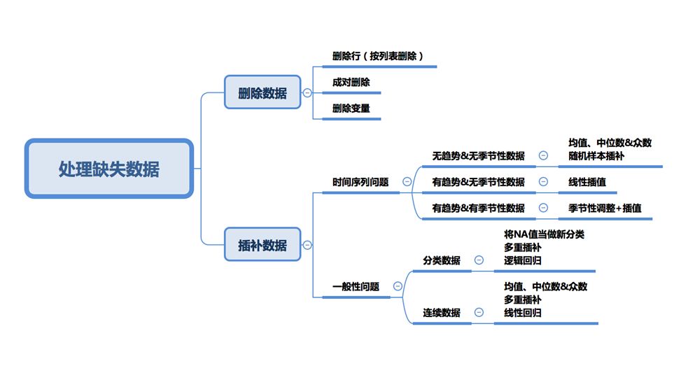
Deletion
Listwise Deletion
Listwise deletion (complete case analysis) deletes a row of observations as long as it contains at least one missing data point. You may only need to delete these observations directly, making analysis easier, especially when the missing data constitutes a small portion of the total data. However, in most cases, this deletion method is not effective because the assumption of completely random missingness (MCAR) is often hard to satisfy. Thus, this deletion method can lead to biased parameters and estimates.
newdata <- na.omit(mydata)
# In python
mydata.dropna(inplace=True)
Pairwise Deletion
In the presence of important variables, pairwise deletion only removes rows of relatively unimportant variables. This helps to ensure sufficient data as much as possible. The advantage of this method is that it can enhance the effectiveness of analysis, but it also has many shortcomings. It assumes that the missing data follows completely random missingness (MCAR). If you use this method, different parts of the final model will have different amounts of observations, making model interpretation very difficult.
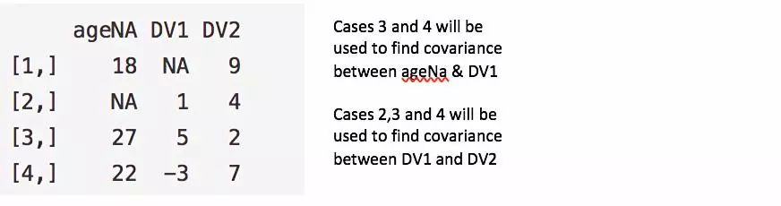
Observation rows 3 and 4 will be used to calculate the covariance between ageNa and DV1; observation rows 2, 3, and 4 will be used to calculate the covariance between DV1 and DV2.
#Pairwise Deletion
ncovMatrix <- cov(mydata, use="pairwise.complete.obs")

#Listwise Deletion
ncovMatrix <- cov(mydata, use="complete.obs")
Variable Deletion
In my opinion, retaining data is always better than discarding it. Sometimes, if more than 60% of the observed data is missing, directly deleting that variable can be acceptable, provided that the variable is not critical. That said, imputing data is always better than directly discarding a variable.
df <- subset(mydata, select = -c(x,z) )
df <- mydata[ -c(1,3:4) ]

In python
del mydata.column_name
mydata.drop('column_name', axis=1, inplace=True)
Time-Series Specific Methods
Last Observation Carried Forward (LOCF) replaces each missing value with the last observed value before it, while Next Observation Carried Backward (NOCB) does the opposite—using the observed value after the missing value for imputation.
These are common methods for analyzing longitudinal repeated measures data that may have missing subsequent observations. Longitudinal data tracks the same sample at different time points. When data has a clear trend, both methods may introduce bias in the analysis and perform poorly.
Linear interpolation. This method is suitable for time series with some trend but no seasonality.
Seasonal adjustment + linear interpolation. This method is suitable for data with trend and seasonality.
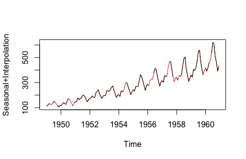
Seasonal + interpolation method
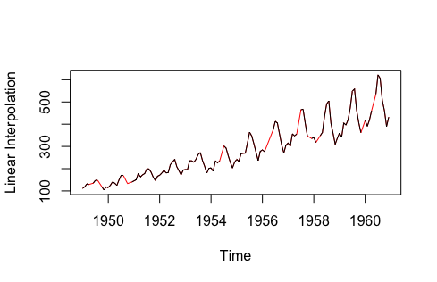
Linear interpolation method
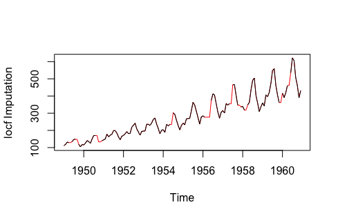
LOCF imputation method
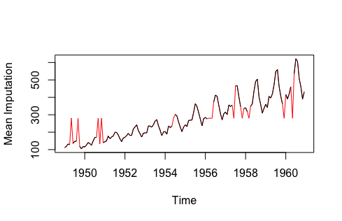
Mean imputation method
Note: The above data is sourced from the imputeTS library’s tsAirgap; imputed data is highlighted in red.
library(imputeTS)

na.random(mydata)                  # Random Imputation
na.locf(mydata, option = "locf")   # Last Obs. Carried Forward
na.locf(mydata, option = "nocb")   # Next Obs. Carried Backward
na.interpolation(mydata)           # Linear Interpolation
na.seadec(mydata, algorithm = "interpolation") # Seasonal Adjustment then Linear Interpolation
Mean, Median, and Mode
Calculating the overall mean, median, or mode is a very basic imputation method and is the only one that does not utilize time series characteristics or variable relationships. This method is very quick to compute, but it has obvious drawbacks. One of the drawbacks is that mean imputation reduces the variation (variance) in the data.
library(imputeTS)

na.mean(mydata, option = "mean")   # Mean Imputation
na.mean(mydata, option = "median") # Median Imputation
na.mean(mydata, option = "mode")   # Mode Imputation

In Python
from sklearn.preprocessing import Imputer
values = mydata.values
imputer = Imputer(missing_values='NaN', strategy='mean')
transformed_values = imputer.fit_transform(values)

# strategy can be changed to "median" and “most_frequent”
Linear Regression
First, using the correlation coefficient matrix can select some predictor variables for the missing data variables. From this, choose the most reliable predictor variables and use them as independent variables in the regression equation. The variables with missing data are used as dependent variables. The rows of observations that have complete data for the independent variables are used to generate the regression equation; then, this equation is used to predict the missing data points. In the iterative process, we insert the values of the missing data variables and then use all data rows to predict the dependent variable. Repeat these steps until the predicted values of this step and the last step are nearly the same, i.e., convergence.
This method theoretically provides a good estimate of the missing data. However, it has several drawbacks that may outweigh its advantages. First, because the replacement values are predicted based on other variables, they tend to combine too well, thus reducing the standard deviation. We must also assume that there is a linear relationship between the variables used in the regression—which in reality may not be the case.
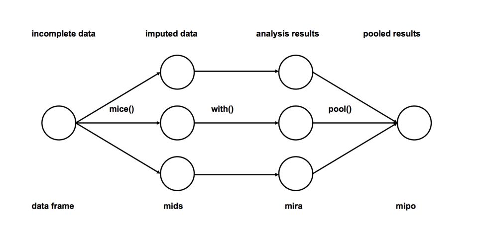
Multiple Imputation
1. Imputation: The incomplete dataset’s missing observations are estimated and filled in m times (in the image, m=3). Note that the filled values are extracted from some distribution. Simulated random draws do not include the uncertainty of the model parameters. A better approach is to use Markov Chain Monte Carlo simulation (MCMC). This step will generate m complete datasets.
2. Analysis: Analyze each of the m complete datasets separately.
3. Combination: Combine the results of the m analyses into the final result.
Source:
http://www.stefvanbuuren.nl/publications/mice%20in%20r%20-%20draft.pdf
# We will be using mice library in r
library(mice)
# Deterministic regression imputation via mice
imp <- mice(mydata, method = "norm.predict", m = 1)

# Store data
data_imp <- complete(imp)

# Multiple Imputation
imp <- mice(mydata, m = 5)

#build predictive model
fit <- with(data = imp, lm(y ~ x + z))

#combine results of all 5 models
combine <- pool(fit)
This is the optimal imputation method so far because it is very easy to use and it does not introduce bias if the imputation model is correct.
Imputation for Categorical Variables
1. Mode imputation can be a method, but it definitely introduces bias.
2. Missing values can be treated as a separate categorical category. We can create a new category for them and use it. This is the simplest method.
3. Predictive models: Here we create a predictive model to estimate the values used to replace the missing data locations. In this case, we split the dataset into two groups: one group excludes the variables with missing data (training group), while the other group includes the missing variables (testing group). We can use methods like logistic regression and ANOVA for prediction.
4. Multiple imputation.
KNN (K-Nearest Neighbors)
There are many machine learning methods available for data imputation, such as XGBoost and Random Forest, but here we discuss the KNN method because it is widely used. In this method, we select k “neighbors” based on some distance measure, and their mean is used to impute the missing data. This method requires us to choose the value of k (the number of nearest neighbors) and the distance measure. KNN can predict both discrete attributes (the most common value among k neighbors) and continuous attributes (the mean of k neighbors).
Depending on the data type, the distance measures can vary:
1. Continuous data: The most commonly used distance measures are Euclidean distance, Manhattan distance, and cosine distance.
2. Categorical data: Hamming distance is commonly used in this case. For all categorical attributes, if the values of two data points differ, the distance increases by one. The Hamming distance actually corresponds to the number of different attribute values.
One of the most attractive features of the KNN algorithm is that it is easy to understand and implement. Its non-parametric nature is advantageous in cases where some data are very “unusual”.
A significant drawback of the KNN algorithm is that it becomes very time-consuming when analyzing large datasets, as it searches the entire dataset for similar data points. Additionally, in high-dimensional datasets, the difference between the nearest and farthest neighbors becomes very small, thus reducing the accuracy of KNN.
library(DMwR)
knnOutput <- knnImputation(mydata)

In python
from fancyimpute import KNN

# Use 5 nearest rows which have a feature to fill in each row's missing features
knnOutput = KNN(k=5).complete(mydata)
Among the methods mentioned, multiple imputation and KNN are the most widely used, with the former usually being preferred due to its simplicity.
Source: Reproduced from Big Data Digest, compiled by Zhang Qiuyue, Hu Jia, and Xia Yawen. Copyright belongs to the authors.
[60 Classic Theories Essential for Management] The green book is here!Consolidate the systematic theoretical foundation of management!Help improve management thinking level!Free Limited edition! Limited to 500 copies! Reply in the background with [Pocket Book] to receive~