This article collects and organizes some common anomaly detection methods available on the public internet (with sources and code). Any shortcomings are welcome to be criticized and corrected.

1. Distribution-Based Methods
1. 3sigma
Based on the normal distribution, the 3sigma criterion considers data points exceeding 3 sigma to be outliers.

def three_sigma(s):
    mu, std = np.mean(s), np.std(s)
    lower, upper = mu-3*std, mu+3*std
    return lower, upper
2. Z-score
The Z-score is a standard score that measures the distance of a data point from the mean; if A differs from the mean by 2 standard deviations, the Z-score is 2. When using a Z-score of 3 as a threshold to eliminate outliers, it is equivalent to 3sigma.
def z_score(s):
  z_score = (s - np.mean(s)) / np.std(s)
  return z_score
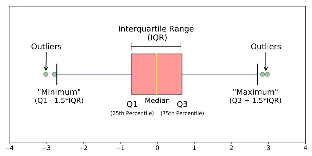
3. Boxplot
The boxplot method identifies outliers based on the interquartile range (IQR).
def boxplot(s):
    q1, q3 = s.quantile(.25), s.quantile(.75)
    iqr = q3 - q1
    lower, upper = q1 - 1.5*iqr, q3 + 1.5*iqr
    return lower, upper
4. Grubbs’ Test
Source:
[1] Overview of Anomaly Detection Algorithms in Time Series Prediction Competitions – Yu Yu Yu and Yu, Zhihu: https://zhuanlan.zhihu.com/p/336944097 [2] Outlier Removal Grid Calculator – Statistics Needed by Data Analysts: Anomaly Detection – weixin_39974030, CSDN: https://blog.csdn.net/weixin_39974030/article/details/112569610
Grubbs’ Test is a hypothesis testing method commonly used to test for a single outlier in a univariate dataset Y that follows a normal distribution. If there is an outlier, it must be the maximum or minimum value in the dataset. The null hypothesis and alternative hypothesis are as follows:
-
H0: There are no outliers in the dataset
-
H1: There is one outlier in the dataset
Using Grubbs’ test requires the population to be normally distributed. The algorithm process is as follows: 1. Sort the sample from smallest to largest 2. Calculate the sample mean and deviation 3. Calculate the difference between min/max and mean; the larger one is the suspicious value 4. Calculate the z-score (standard score) of the suspicious value; if it exceeds the Grubbs critical value, it is an outlier. The Grubbs critical value can be found in tables and is determined by two values: the detection level α (the stricter, the smaller) and the sample size n. Exclude outliers and repeat steps 1-4 for the remaining sequence [1]. Detailed calculation examples can be referenced.
from outliers import smirnov_grubbs as grubbs
print(grubbs.test([8, 9, 10, 1, 9], alpha=0.05))
print(grubbs.min_test_outliers([8, 9, 10, 1, 9], alpha=0.05))
print(grubbs.max_test_outliers([8, 9, 10, 1, 9], alpha=0.05))
print(grubbs.max_test_indices([8, 9, 10, 50, 9], alpha=0.05))
Limitations: 1. Can only detect univariate data 2. Cannot accurately output normal intervals 3. Its judgment mechanism is “one by one elimination”, so each outlier must be calculated through the entire process individually, which is inefficient for large datasets. 4. It is necessary to assume that the data follows a normal or nearly normal distribution.
2. Distance-Based Methods
1. KNN
Source:
[3] Anomaly Detection Algorithm of K Nearest Neighbors – Xiao Wu Ge Talks Risk Control, Zhihu: https://zhuanlan.zhihu.com/p/501691799
It calculates the average distance from each sample point to its K nearest samples and compares the calculated distance with the threshold. If it exceeds the threshold, it is considered an outlier. The advantage is that it does not require assumptions about the distribution of the data, while the disadvantage is that it can only find global outliers and cannot find local outliers.
from pyod.models.knn import KNN

# Initialize detector clf
clf = KNN(method='mean', n_neighbors=3, )
clf.fit(X_train)
# Return classification labels on training data (0: normal value, 1: outlier)
y_train_pred = clf.labels_
# Return outliers on training data (the larger the score, the more abnormal)
y_train_scores = clf.decision_scores_
3. Density-Based Methods
1. Local Outlier Factor (LOF)
Source:
[4] Understand Anomaly Detection LOF Algorithm (Python Code) – Dong Ge Takes Off, Zhihu: https://zhuanlan.zhihu.com/p/448276009
LOF is a classic density-based algorithm (Breuning et al. 2000) that assigns an outlier factor LOF to each data point based on neighborhood density to determine whether the data point is an outlier. Its advantage is that it can quantify the degree of abnormality (outlierness) of each data point.
The local relative density of point P (local outlier factor) is the ratio of the average local reachability density of points in the neighborhood of point P to the local reachability density of point P itself, which is: the local reachability density of point P = the inverse of the average reachability distance of P’s nearest neighbors. The distance is larger, and the density is smaller. The k-th reachability distance from point P to point O = max(distance to the k nearest neighbors of point O, distance from point P to point O).
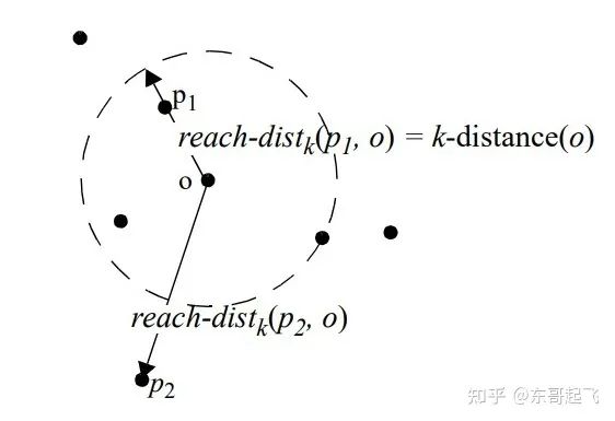
The k-nearest neighbor distance of point O is the distance between the k-th nearest point and point O. Overall, the LOF algorithm process is as follows:
-
For each data point, calculate its distance to all other points and sort them from nearest to farthest;
-
For each data point, find its K-Nearest-Neighbor and calculate the LOF score.
from sklearn.neighbors import LocalOutlierFactor as LOF

X = [[-1.1], [0.2], [100.1], [0.3]]
clf = LOF(n_neighbors=2)
res = clf.fit_predict(X)
print(res)
print(clf.negative_outlier_factor_)
2. Connectivity-Based Outlier Factor (COF)
Source:
[5] Nowak-Brzezińska, A., & Horyń, C. (2020). Outliers in rules – the comparison of LOF, COF, and KMEANS algorithms. *Procedia Computer Science*, *176*, 1420-1429. [6] Machine Learning Learning Notes Series (98): Analysis Based on Connectivity Outlier Factor – Liu Zhihao (Chih-Hao Liu)
COF is a variant of LOF. Compared to LOF, COF can handle outliers in low-density areas. The local density of COF is calculated based on the average chain distance. Initially, we will calculate the k-nearest neighbor for each point. Then we will calculate the Set based nearest Path for each point, as shown in the figure:
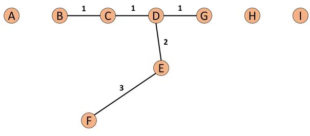
Assuming we set k=5, the neighbors of F are B, C, D, E, and G. The nearest point to F is E, so the first element of the SBN Path is F, the second is E. The nearest point to E is D, so the third element is D, and the nearest points to D are C and G, making the fourth and fifth elements C and G, and finally, the nearest point to C is B, making the sixth element B. Thus, the entire SBN Path for F is {F, E, D, C, G, C, B}. For the distances corresponding to the SBN Path e={e1, e2, e3,…,ek}, according to the above example, e={3,2,1,1,1}. Therefore, we can say that if we want to calculate the SBN Path of point p, we just need to compute the minimum spanning tree of the graph formed by point p and all its neighbor points, and then execute the shortest path algorithm starting from point p to obtain our SBN Path. Next, we have the SBN Path and will continue to calculate the chain distance for point p: having the ac_distance allows us to calculate COF:
# https://zhuanlan.zhihu.com/p/362358580
from pyod.models.cof import COF
cof = COF(contamination=0.06,  # the proportion of outliers
          n_neighbors=20,      # number of neighbors
        )
cof_label = cof.fit_predict(iris.values)  # Iris dataset
print("Number of detected outliers:", np.sum(cof_label == 1))
3. Stochastic Outlier Selection (SOS)
Source:
[7] Anomaly Detection SOS Algorithm – Hu Guangyue, Zhihu: https://zhuanlan.zhihu.com/p/34438518
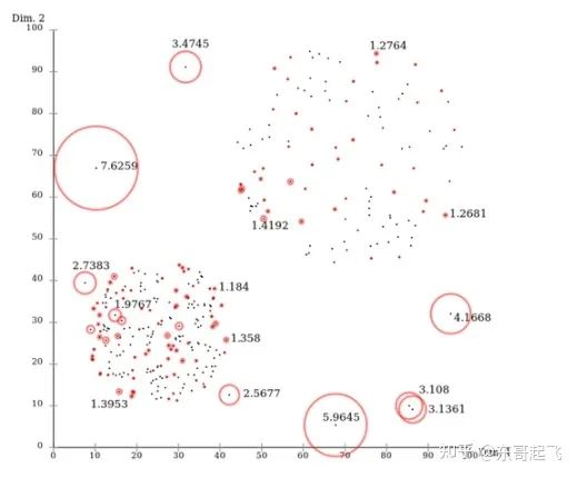
By inputting the feature matrix or dissimilarity matrix into the SOS algorithm, it returns an anomaly probability value vector (one for each point). The idea of SOS is: when a point has a low affinity with all other points, it is considered an outlier.
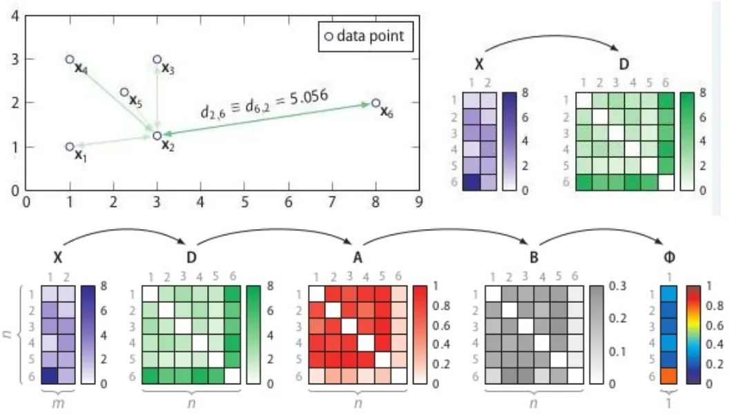
The process of SOS is:
-
Calculate the dissimilarity matrix D;
-
Calculate the affinity matrix A;
-
Calculate the binding probability matrix B;
-
Calculate the anomaly probability vector.
The dissimilarity matrix D is a measure of distance between each pair of samples, such as Euclidean distance or Hamming distance. The affinity matrix reflects the variance of the measured distances, as shown in Figure 7; point P has the highest density and the lowest variance; point Q has the lowest density and the highest variance. The binding probability matrix is obtained by normalizing the affinity matrix row-wise, as shown in Figure 8.

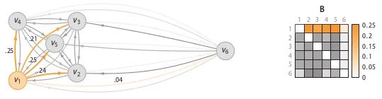
After obtaining the binding probability matrix, the anomaly probability value for each point is calculated using the following formula. When a point has a low affinity with all other points, it is considered an outlier.
# Ref: https://github.com/jeroenjanssens/scikit-sos
import pandas as pd
from sksos import SOS
iris = pd.read_csv("http://bit.ly/iris-csv")
X = iris.drop("Name", axis=1).values

detector = SOS()
iris["score"] = detector.predict(X)
iris.sort_values("score", ascending=False).head(10)
4. Clustering-Based Methods
1. DBSCAN
The DBSCAN algorithm (Density-Based Spatial Clustering of Applications with Noise) has the following inputs and outputs: isolated points that cannot form clusters are considered outliers (noise points).
-
Input: dataset, neighborhood radius Eps, threshold MinPts for the number of data objects in the neighborhood;
-
Output: density-connected clusters.
Processing steps are as follows:
-
Select any data object point p from the dataset;
-
If the selected data object point p is a core point for parameters Eps and MinPts, find all data object points that are density reachable from p to form a cluster;
-
If the selected data object point p is a border point, select another data object point;
-
Repeat steps 2 and 3 until all points are processed.
# Ref: https://zhuanlan.zhihu.com/p/515268801
from sklearn.cluster import DBSCAN
import numpy as np
X = np.array([[1, 2], [2, 2], [2, 3],
              [8, 7], [8, 8], [25, 80]])
clustering = DBSCAN(eps=3, min_samples=2).fit(X)

clustering.labels_
array([ 0,  0,  0,  1,  1, -1])
# 0, 0, 0: indicates that the first three samples are grouped into one cluster
# 1, 1: indicates that the next two are grouped into one cluster
# -1: indicates that the last one is an outlier, not belonging to any cluster
5. Tree-Based Methods
1. Isolation Forest (iForest)
Source:
[8] Anomaly Detection Algorithm – Isolation Forest Analysis – Risk Control Big Fish, Zhihu: https://zhuanlan.zhihu.com/p/74508141 [9] Isolation Forest – An Algorithm for Anomaly Detection – Xiao Wu Ge Talks Risk Control, Zhihu: https://zhuanlan.zhihu.com/p/484495545 [10] Isolation Forest Reading – Mark_Aussie, Blog: https://blog.csdn.net/MarkAustralia/article/details/120181899
The term “isolation” in Isolation Forest refers to “isolating outliers from all samples”. The original text in the paper states “separating an instance from the rest of the instances”. We cut a data space with a random hyperplane; one cut can generate two subspaces. Next, we randomly select hyperplanes to cut the two subspaces obtained from the first step, and this process continues until each subspace contains only one data point. We can find that dense clusters require many cuts to stop cutting, meaning that each point exists in a subspace, while sparse points tend to stop in a subspace early. Therefore, the entire algorithm idea of Isolation Forest is: abnormal samples are more likely to quickly fall into leaf nodes or, in other words, abnormal samples are closer to the root node on the decision tree. Randomly select m features and split data points by randomly choosing a value between the maximum and minimum of the selected features. The division of observations is recursively repeated until all observations are isolated.
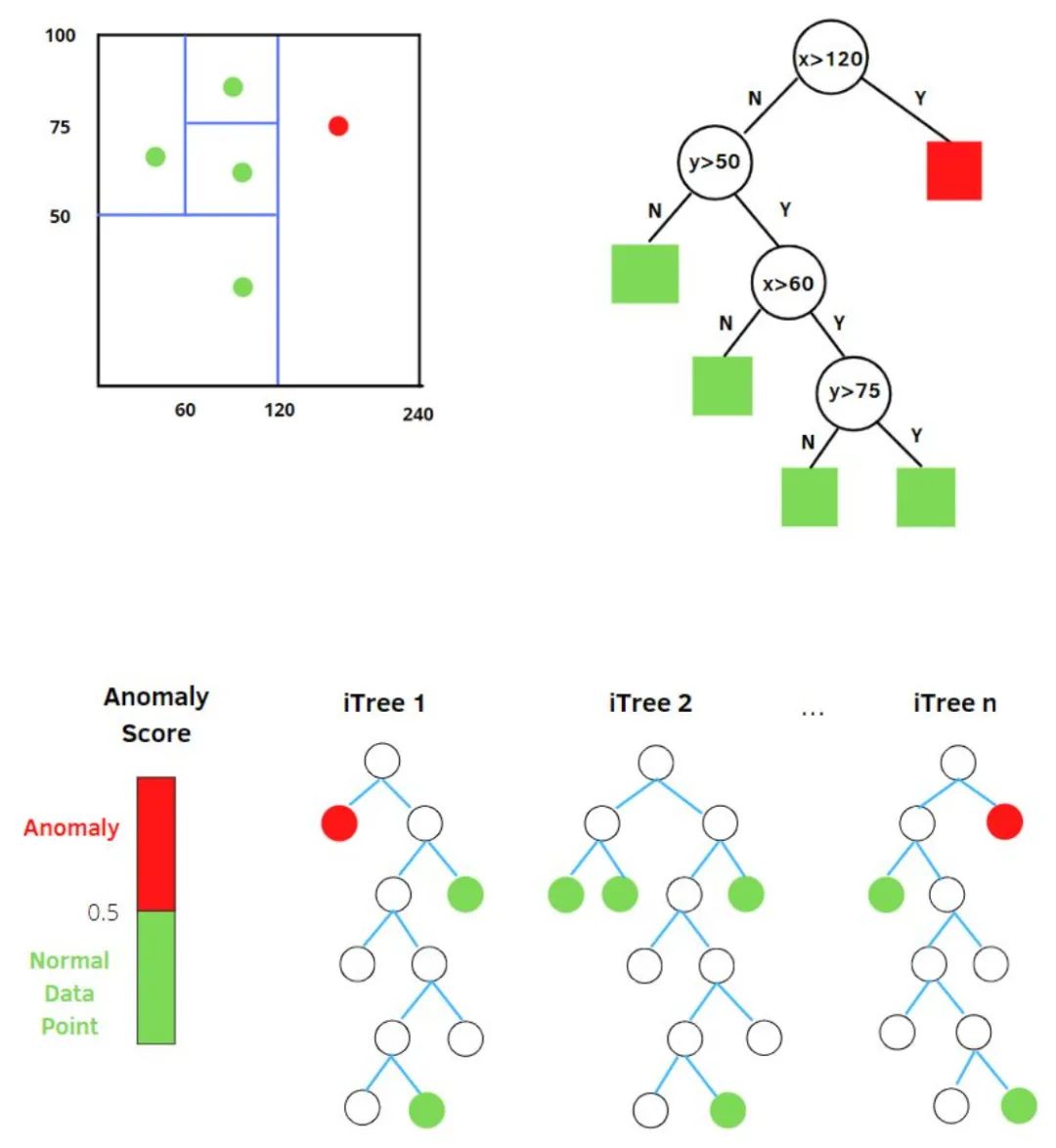
After obtaining t isolation trees, the training of a single tree is complete. Next, we can use the generated isolation trees to evaluate test data, that is, to calculate anomaly scores s. For each sample x, we need to comprehensively calculate the results of each tree using the following formula:
-
h(x): Path Length of the sample on iTree;
-
E(h(x)): The mean Path Length of the sample on t iTrees;
-
h(x): The estimated average path length of a successful search in a binary search tree (BST) for the sample x (the mean h(x) estimated for external terminal nodes is equivalent to the BST’s last successful search).
The exponent value ranges from (−∞,0), therefore the s value ranges from (0,1). When the Path Length is smaller, s is closer to 1, which means the probability of the sample being an outlier is greater.
# Ref: https://zhuanlan.zhihu.com/p/484495545
from sklearn.datasets import load_iris
from sklearn.ensemble import IsolationForest

data = load_iris(as_frame=True)
X,y = data.data,data.target
df = data.frame

# Model training
iforest = IsolationForest(n_estimators=100, max_samples='auto',
                          contamination=0.05, max_features=4,
                          bootstrap=False, n_jobs=-1, random_state=1)

# fit_predict function trains and predicts together to get whether the model is anomalous, -1 for anomaly, 1 for normal
df['label'] = iforest.fit_predict(X)

# The decision_function can yield anomaly scores
df['scores'] = iforest.decision_function(X)
6. Dimensionality Reduction Methods
1. Principal Component Analysis (PCA)
Source:
[11] Machine Learning – Anomaly Detection Algorithm (III): Principal Component Analysis – Liu Tengfei, Zhihu: https://zhuanlan.zhihu.com/p/29091645 [12] Anomaly Detection – PCA Algorithm Implementation – CC Si SS, Zhihu: https://zhuanlan.zhihu.com/p/48110105
PCA in anomaly detection generally has two approaches: (1) Mapping the data to a low-dimensional feature space and checking the deviation of each data point from the others in different dimensions; (2) Mapping the data to a low-dimensional feature space and then remapping back to the original space, attempting to reconstruct the original data using low-dimensional features and observing the size of reconstruction errors. PCA performs eigenvalue decomposition, which yields:
-
Eigenvectors: Reflect the different directions of variance change in the original data;
-
Eigenvalues: The magnitude of variance in the corresponding direction of the data.
Thus, the maximum eigenvalue corresponds to the direction of maximum variance in the data, while the minimum eigenvalue corresponds to the direction of minimum variance. The variance change of the original data in different directions reflects its intrinsic characteristics. If a single data sample deviates significantly from the overall data sample characteristics, for instance, deviating greatly in certain directions compared to other data samples, it may indicate that this data sample is an outlier. In the first approach mentioned, the anomaly score of a sample is the degree of deviation of that sample in all directions:where is the distance of the sample in the reconstruction space from the eigenvector. If there are sample points deviating far from the principal components, the score will be larger, indicating a high degree of deviation and a high anomaly score. The eigenvalue is used for normalization to make the degrees of deviation in different directions comparable. There are two ways to select eigenvectors (i.e., benchmarks for measuring anomalies) when calculating anomaly scores:
-
Consider the deviations in the directions of the first k eigenvectors: the first few eigenvectors often correspond directly to several features in the original data, and data samples with significant deviations in the directions of the first few eigenvectors are often extreme points in those features in the original data.
-
Consider the deviations in the directions of the last r eigenvectors: the last r eigenvectors usually represent linear combinations of several original features, and the variance after linear combinations is relatively small, reflecting some relationship between these features. Data samples with significant deviations in the last few feature directions indicate discrepancies from expected behavior in the corresponding features in the original data.
Scores greater than threshold C are considered anomalies. In the second approach, PCA extracts the main features of the data; if a data sample is not easily reconstructed, it indicates that the features of this data sample are inconsistent with the overall data sample features, thus it is clearly an outlier:where is the sample reconstructed based on the dimensionality feature vectors. During the reconstruction of data samples based on low-dimensional features, information in the directions of eigenvectors corresponding to smaller eigenvalues is discarded. In other words, reconstruction errors mainly arise from information in the directions of eigenvectors corresponding to smaller eigenvalues. Based on this intuitive understanding, both approaches of PCA for anomaly detection particularly focus on the directions of eigenvectors corresponding to smaller eigenvalues.
# Ref: [https://zhuanlan.zhihu.com/p/48110105]
from sklearn.decomposition import PCA
pca = PCA()
pca.fit(centered_training_data)
transformed_data = pca.transform(training_data)
y = transformed_data

# Calculate anomaly scores
lambdas = pca.singular_values_
M = ((y*y)/lambdas)

# First k eigenvectors and last r eigenvectors
q = 5
print("Explained variance by first q terms: ", sum(pca.explained_variance_ratio_[:q]))
q_values = list(pca.singular_values_ < .2)
r = q_values.index(True)

# Calculate distance sums for each sample point
major_components = M[:,range(q)]
minor_components = M[:,range(r, len(features))]
major_components = np.sum(major_components, axis=1)
minor_components = np.sum(minor_components, axis=1)

# Manually set thresholds c1, c2
components = pd.DataFrame({'major_components': major_components,
                               'minor_components': minor_components})
c1 = components.quantile(0.99)['major_components']
c2 = components.quantile(0.99)['minor_components']

# Create classifier
def classifier(major_components, minor_components):
    major = major_components > c1
    minor = minor_components > c2
    return np.logical_or(major,minor)

results = classifier(major_components=major_components, minor_components=minor_components)
2. AutoEncoder
Source:
[13] Unsupervised Anomaly Detection Using Autoencoder (Python) – SofaSofa.io, Zhihu: https://zhuanlan.zhihu.com/p/46188296 [14] Autoencoder Solving Anomaly Detection Problems (Step-by-Step Code) – Data Like Amber, Zhihu: https://zhuanlan.zhihu.com/p/260882741
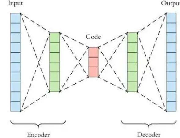
PCA is linear dimensionality reduction, while AutoEncoder is non-linear dimensionality reduction. An AutoEncoder trained on normal data can reconstruct normal samples well, but cannot reconstruct data points that deviate from the normal distribution well, leading to larger reconstruction errors. Therefore, if a new sample is encoded and the reconstruction error exceeds the normal range of errors from encoded and decoded normal data, it is considered anomalous data. It is important to note that the data used to train the AutoEncoder is normal data (i.e., no outliers), so that the distribution range of reconstruction errors can be established. Thus, AutoEncoder is a form of supervised learning for anomaly detection.
# Ref: [https://zhuanlan.zhihu.com/p/260882741]
import tensorflow as tf
from keras.models import Sequential
from keras.layers import Dense

# Normalize data
scaler = preprocessing.MinMaxScaler()
X_train = pd.DataFrame(scaler.fit_transform(dataset_train),
                              columns=dataset_train.columns,
                              index=dataset_train.index)
# Random shuffle training data
X_train.sample(frac=1)
X_test = pd.DataFrame(scaler.transform(dataset_test),
                             columns=dataset_test.columns,
                             index=dataset_test.index)

tf.random.set_seed(10)
act_func = 'relu'
# Input layer:
model=Sequential()
# First hidden layer, connected to input vector X.
model.add(Dense(10,activation=act_func,
                kernel_initializer='glorot_uniform',
                kernel_regularizer=regularizers.l2(0.0),
                input_shape=(X_train.shape[1],)
               )
         )
model.add(Dense(2,activation=act_func,
                kernel_initializer='glorot_uniform'))
model.add(Dense(10,activation=act_func,
                kernel_initializer='glorot_uniform'))
model.add(Dense(X_train.shape[1],
                kernel_initializer='glorot_uniform'))
model.compile(loss='mse',optimizer='adam')
print(model.summary())

# Train model for 100 epochs, batch size of 10:
NUM_EPOCHS=100
BATCH_SIZE=10
history=model.fit(np.array(X_train),np.array(X_train),
                  batch_size=BATCH_SIZE,
                  epochs=NUM_EPOCHS,
                  validation_split=0.05,
                  verbose = 1)

plt.plot(history.history['loss'],
         'b',
         label='Training loss')
plt.plot(history.history['val_loss'],
         'r',
         label='Validation loss')
plt.legend(loc='upper right')
plt.xlabel('Epochs')
plt.ylabel('Loss, [mse]')
plt.ylim([0,.1])
plt.show()

# Check how the reconstruction error distribution of the training set looks to establish the normal error distribution range
X_pred = model.predict(np.array(X_train))
X_pred = pd.DataFrame(X_pred,
                      columns=X_train.columns)
X_pred.index = X_train.index

scored = pd.DataFrame(index=X_train.index)
scored['Loss_mae'] = np.mean(np.abs(X_pred-X_train), axis = 1)
plt.figure()
sns.distplot(scored['Loss_mae'],
             bins = 10,
             kde= True,
            color = 'blue')
plt.xlim([0.0,.5])

# Compare reconstruction error thresholds to identify outliers
X_pred = model.predict(np.array(X_test))
X_pred = pd.DataFrame(X_pred,
                      columns=X_test.columns)
X_pred.index = X_test.index
threshold = 0.3
scored = pd.DataFrame(index=X_test.index)
scored['Loss_mae'] = np.mean(np.abs(X_pred-X_test), axis = 1)
scored['Threshold'] = threshold
scored['Anomaly'] = scored['Loss_mae'] > scored['Threshold']
scored.head()
7. Classification-Based Methods
1. One-Class SVM
Source:
[15] Python Machine Learning Notes: One Class SVM – zoukankan, Blog: http://t.zoukankan.com/wj-1314-p-10701708.html [16] One-Class SVM: SVDD – Zhang Yice, Zhihu: https://zhuanlan.zhihu.com/p/65617987
One-Class SVM is a very simple algorithm that finds a hyperplane to enclose the positive examples in the sample; prediction uses this hyperplane for decisions, with samples inside the hyperplane considered positive and those outside considered negative. In anomaly detection, negative samples can be regarded as outliers.

One-Class SVM can also be derived using SVDD (Support Vector Domain Description). For SVDD, we expect all samples that are not outliers to be positive, and it uses a hypersphere instead of a hyperplane for classification. This algorithm obtains a spherical boundary around the data in feature space, aiming to minimize the volume of this hypersphere, thereby minimizing the impact of outlier data. Assuming the parameters of the generated hypersphere are center o and the corresponding radius r>0, the volume V(r) of the hypersphere is minimized, and the center o is a linear combination of support vectors; similar to traditional SVM methods, we can require that all training data points xi are strictly less than r from the center. However, a slack variable ζi with a penalty coefficient C is also constructed, and the optimization problem is as follows: C adjusts the influence of slack variables; in simple terms, it gives those data points that need slack a certain amount of slack space. If C is small, it allows greater flexibility for outlier points, enabling them to be excluded from the hypersphere. For detailed derivation, refer to sources [15] [16].
from sklearn import svm
# fit the model
clf = svm.OneClassSVM(nu=0.1, kernel='rbf', gamma=0.1)
clf.fit(X)
y_pred = clf.predict(X)
n_error_outlier = y_pred[y_pred == -1].size
8. Prediction-Based Methods
Source:
[17] TS Technology Class: Time Series Anomaly Detection – Time Series Person, Article: https://mp.weixin.qq.com/s/9TimTB_ccPsme2MNPuy6uA
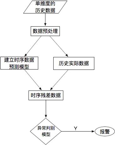
For a single time series data, by comparing the predicted time series curve with the actual data, the residual of each point can be calculated, and the residual sequence can be modeled using methods such as KSigma or quantiles for anomaly detection. The specific process is as follows:
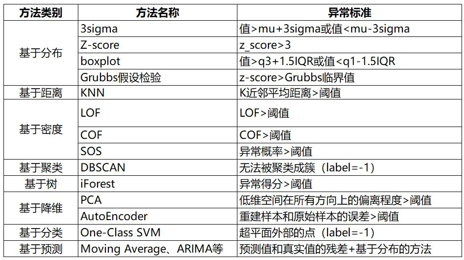
9. Summary
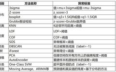
The summary of anomaly detection methods is as follows:

References[1] Overview of Anomaly Detection Algorithms in Time Series Prediction Competitions – Yu Yu Yu and Yu, Zhihu: https://zhuanlan.zhihu.com/p/336944097[2] Outlier Removal Grid Calculator – Statistics Needed by Data Analysts: Anomaly Detection – weixin_39974030, CSDN: https://blog.csdn.net/weixin_39974030/article/details/112569610[3] Anomaly Detection Algorithm of K Nearest Neighbors – Xiao Wu Ge Talks Risk Control, Zhihu: https://zhuanlan.zhihu.com/p/501691799[4] Understand Anomaly Detection LOF Algorithm (Python Code) – Dong Ge Takes Off, Zhihu: https://zhuanlan.zhihu.com/p/448276009[5] Nowak-Brzezińska, A., & Horyń, C. (2020). Outliers in rules – the comparison of LOF, COF, and KMEANS algorithms. *Procedia Computer Science*, *176*, 1420-1429.[6] Machine Learning Learning Notes Series (98): Analysis Based on Connectivity Outlier Factor – Liu Zhihao (Chih-Hao Liu)[7] Anomaly Detection SOS Algorithm – Hu Guangyue, Zhihu: https://zhuanlan.zhihu.com/p/34438518[8] Anomaly Detection Algorithm – Isolation Forest Analysis – Risk Control Big Fish, Zhihu: https://zhuanlan.zhihu.com/p/74508141[9] Isolation Forest – An Algorithm for Anomaly Detection – Xiao Wu Ge Talks Risk Control, Zhihu: https://zhuanlan.zhihu.com/p/484495545[10] Isolation Forest Reading – Mark_Aussie, Blog: https://blog.csdn.net/MarkAustralia/article/details/120181899[11] Machine Learning – Anomaly Detection Algorithm (III): Principal Component Analysis – Liu Tengfei, Zhihu: https://zhuanlan.zhihu.com/p/29091645[12] Anomaly Detection – PCA Algorithm Implementation – CC Si SS, Zhihu: https://zhuanlan.zhihu.com/p/48110105[13] Unsupervised Anomaly Detection Using Autoencoder (Python) – SofaSofa.io, Zhihu: https://zhuanlan.zhihu.com/p/46188296[14] Autoencoder Solving Anomaly Detection Problems (Step-by-Step Code) – Data Like Amber, Zhihu: https://zhuanlan.zhihu.com/p/260882741[15] Python Machine Learning Notes: One Class SVM – zoukankan, Blog: http://t.zoukankan.com/wj-1314-p-10701708.html[16] One-Class SVM: SVDD – Zhang Yice, Zhihu: https://zhuanlan.zhihu.com/p/65617987[17] TS Technology Class: Time Series Anomaly Detection – Time Series Person, Article: https://mp.weixin.qq.com/s/9TimTB_ccPsme2MNPuy6uA
--End--

If you want to buy books at a discount, please check: Discount Book Purchase Channels