
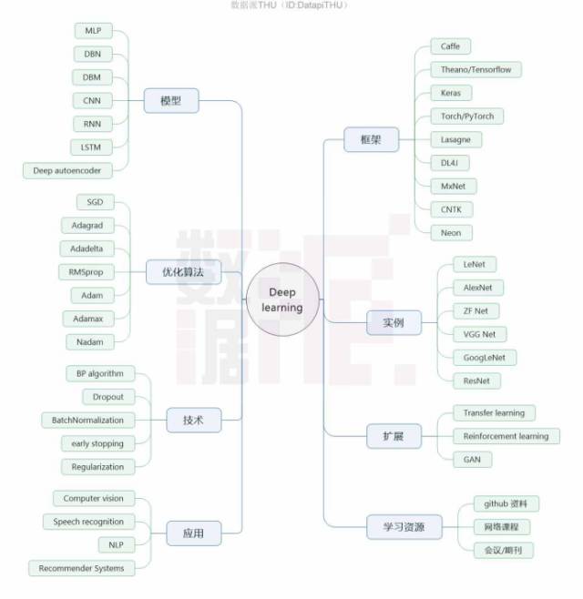
Figure1. Deep Learning Mind Map
Introduction
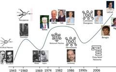
The concept of deep learning can be traced back to the field of cybernetics between 1940 and 1960. It later developed into connectionism during the 1980s and 1990s, with the third wave of development beginning in 2006 with the expansion of artificial neural networks, evolving into the highly popular deep learning we know today (Figure 2). The rise and development of deep learning is quite natural; classical machine learning methods require a deep understanding of specific problems or data, necessitating manual feature extraction to solve problems effectively. However, manual feature extraction is complex and time-consuming. Therefore, methods that can automatically learn features from data have great potential for development, and these methods fall under the category known as representation learning.
Researchers soon discovered that deep representation learning models could abstract more complex features from simple features, which is more conducive to final classification and discrimination, leading to the development of deep learning frameworks. Of course, the advancement of deep learning is also inseparable from the development of algorithms like BP, computational hardware, and data scale. Deep learning can be understood as a framework of machine learning, corresponding to classical shallow learning methods like SVM and LR, representing the second major stage of machine learning development. Currently, deep learning plays a very important role in the field of artificial intelligence, and it can even be said that the development of artificial intelligence benefits greatly from the advancement of deep learning. Due to the close relationship between them, non-professionals often confuse deep learning, artificial intelligence, representation learning, and machine learning concepts.
Furthermore, in recent years, the rapid development of artificial intelligence and the internet has brought significant attention to the technologies behind them, with deep learning receiving the most focus due to its powerful capabilities and relatively low entry barriers. This article aims to introduce readers to deep learning from multiple aspects, including models, technologies, optimization methods, commonly used frameworks and platforms, applications, and examples, while also recommending some learning resources for deep learning at the end of the article.
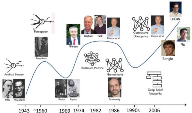
Figure 2. Development of Neural Networks
What is Deep Learning?
As mentioned in the introduction, deep learning is a framework of machine learning and one of the foundational technologies of artificial intelligence. The relationship between deep learning, artificial intelligence, and representation learning can be seen in Figure 3, where machine learning is a method to achieve artificial intelligence, and representation learning is a framework of machine learning, with deep learning included within representation learning.
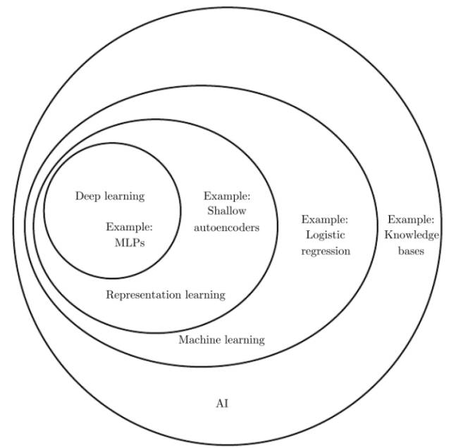
Figure 3. Positioning of Deep Learning (Image Source: Ian Goodfellow et al. Deep Learning.)
Deep learning models can automatically learn features from input data for training. The shallow structures of the model extract simple features, while the deeper structures extract more abstract features based on the features obtained from the shallow layers. This learning method distinguishes deep learning from traditional machine learning and ordinary representation learning models. Figure 4 illustrates the learning methods of different machine learning approaches.
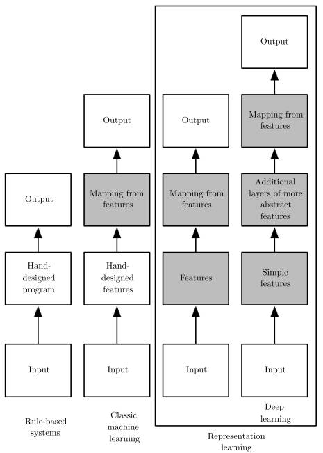
Figure 4. Feature Learning Process in Deep Learning (Image Source: Ian Goodfellow et al. Deep Learning.)
So, in what aspects does the depth of deep learning manifest? Currently, there are two main viewpoints on this issue: the first viewpoint holds that the depth of deep learning is determined by the length of the computational graph, meaning the length of the path of computations from input to output. For this viewpoint, how to define the computation unit is crucial, yet there is currently no unified definition of computation units; the second viewpoint suggests that the depth of deep learning is determined by the depth of the structural diagram that describes the conceptual relationships between input and output, meaning the structural depth of the defined model. However, this structural depth often does not align with the computational depth. These two viewpoints provide two perspectives for understanding deep learning, and we can interpret it as either the depth of model structure or the depth of computation. The author believes that this does not affect the understanding of the essence of deep learning.
Common Models
As mentioned multiple times, deep learning is a framework of machine learning, so what specific models exist within this framework? Below are some common deep learning models.
MLP:
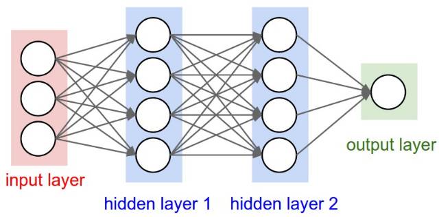
MLP (Multilayer Perceptron) is a typical deep learning model, also known as a feedforward deep network, primarily composed of a neural network with multiple layers (Figure 5). It includes an input layer, hidden layers, and an output layer, where all layers are fully connected. Except for the input layer, each neuron in other layers contains an activation function. Thus, MLP can be seen as a function mapping inputs to outputs, consisting of multiple layers of product operations and activation operations. MLP calculates the final loss function value through forward propagation and then computes the gradient using the backpropagation algorithm (BP), optimizing the model parameters using gradient descent. The emergence of MLP solved the problem that perceptrons could not learn the XOR function, restoring confidence in neural networks.
DBN and DBM:
DBN (Deep Belief Network) is also a classic deep learning model proposed relatively early. DBN is built based on the RBM (Restricted Boltzmann Machine) model. More specifically, the DBN model can be seen as composed of multiple RBM structures and a BP layer, with its training process gradually training each RBM structure from front to back, optimizing each RBM’s hidden layer to optimize the overall network. Notably, in the DBN structure, only the last two layers are undirected connected, while all other layers have directional connections, which is an important feature distinguishing DBN from the later DBM.
DBM (Deep Boltzmann Machine) is also a deep model based on RBM, differing from RBM in that it has multiple hidden layers (RBM only has one hidden layer). The training method of DBM is also to treat the entire network structure as multiple RBMs and then train each RBM one by one from front to back, optimizing the overall model. In the DBM model, all connections between adjacent layers are undirected. In both DBN and DBM models, there are no connections between nodes in different layers, and the nodes are independent of each other.
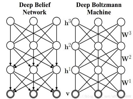
Figure 6. DBN and DBM Model Diagram (Hinton et al. 2006)
CNN:
CNN (Convolutional Neural Network) is a type of feedforward artificial neural network model, officially proposed by Yann LeCun et al. in 1998. Its typical network structure includes convolution layers, pooling layers, and fully connected layers. The diagram below (Figure 7) shows a typical CNN structure (LeNet-5). Given an image (a training sample) as input, multiple convolution operators sequentially scan the input image, and the scan results are activated through an activation function to obtain feature maps. Then, pooling operators are used to downsample the feature maps, and the output results serve as input for the next layer. After passing through all convolution and pooling layers, the results are further processed using a fully connected neural network, with the final results output at the output layer.
The CNN model emphasizes the intermediate convolution process, which significantly reduces the number of model parameters through weight sharing, allowing the model to be trained more efficiently without losing power. The CNN model is very flexible; its structure can be designed arbitrarily under reasonable conditions. For example, pooling layers can be added after multiple convolution layers. Due to this flexibility, CNNs are widely applied in various tasks with significant effectiveness, such as AlexNet, GoogLeNet, VGGNet, and ResNet, which will be introduced later.
Of course, this flexibility also means that the structure of CNN itself becomes a hyperparameter, making it difficult to ensure that the model used for a specific task is optimal. In practical applications, CNNs are more often used to process grid data, such as images, where the convolution process can play a greater role. However, CNNs can also handle various types of tasks, including image recognition, natural language processing, video analysis, drug discovery, and gaming.
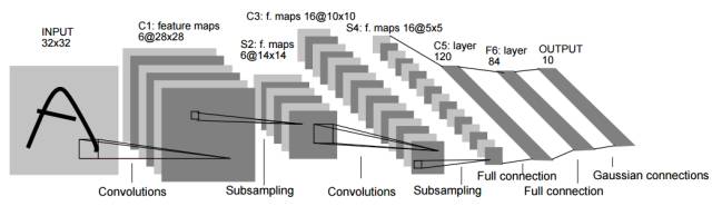
Figure 7. Typical Structure and Operation Process of CNN (Yann LeCun et al. 1998)
RNN:
RNN (Recurrent Neural Network) is a type of neural network model used for processing sequential data. A typical RNN model generally consists of three types of neurons: input, hidden, and output. The input units are only connected to the hidden units, while the hidden units are connected to the output, the previous hidden unit, and the next hidden unit. The output units only receive inputs from the hidden units. During the training process of RNN, it is generally necessary to learn and optimize three types of parameters, namely the weights mapping inputs to the hidden layer, the transition weights between hidden units, and the weights mapping hidden units to outputs.
As shown in Figure 8, the typical RNN structure and computation process. In the computation process of RNN, information from the earlier parts of the sequential data is passed through hidden units to later parts, so that information from earlier parts is considered during the computation of later parts, simulating the dependency relationships between different parts of the sequence. It is evident that RNN models are more suitable for sequential data, especially context-dependent sequences, making RNN widely used in sentiment analysis, image captioning, machine translation, and more. It is worth noting that RNN structures may vary in different tasks; for example, in image captioning scenarios, RNN is structured as one-to-many, while in sentiment analysis, it is structured as many-to-one (Figure 9).
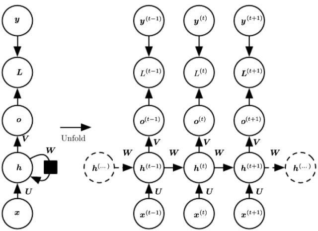
Figure 8. RNN Structure and Computation Process (Ian Goodfellow et al. Deep Learning.)
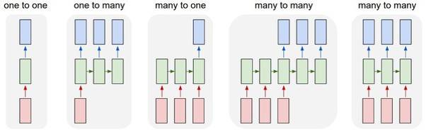
Figure 9. RNN Structures in Different Application Scenarios. From left to right, they correspond to image classification, image captioning, sentiment analysis, machine translation, and video classification.
LSTM:
LSTM (Long Short-Term Memory) model is essentially also an RNN model, differing from RNN in that it introduces the concept of cell state and can add or remove information from the cell state through gates. Additionally, LSTM can form closed loops through gates (Figure 10), allowing it to overcome the weakness of RNN in effectively remembering long-term information. Figure 10 illustrates a common LSTM unit, which consists of input, input gate, forget gate, state, output gate, and output.
In the LSTM model, what is referred to as a gate is essentially a function operation; for example, the input gate can be the sigmoid function operation of all inputs after weight multiplication. For a sequential data sample, the current input node will integrate the hidden output information of the previous node, outputting the current node’s hidden output information through multiple different gate operations, while simultaneously integrating it with the previous node’s cell state information to output the current node’s cell state information (Figure 11). Since LSTM is a special type of RNN model, it can also be applied in many scenarios where RNN can be used, such as sentiment analysis, image captioning, etc. Of course, there are many variants of LSTM, and they perform differently in various tasks, which also requires some understanding when applying them.
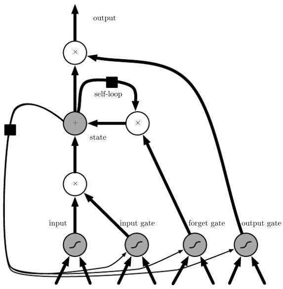
Figure 10. LSTM Structure Diagram (Ian Goodfellow et al. Deep Learning.)
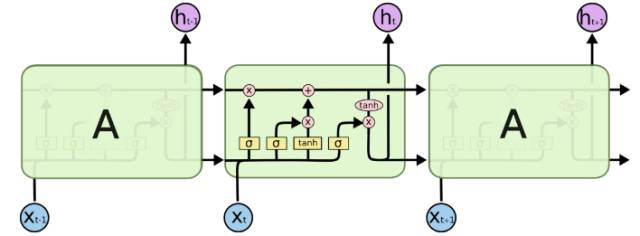
Figure 11. LSTM Data Flow Diagram (Image from the Internet)
Deep Autoencoder:
Autoencoder is a type of neural network where the input layer and output layer represent the same meaning and have the same number of neurons. The learning process of autoencoder involves encoding the input and then decoding it to reconstruct the input as output, with the intermediate representation generated by encoding the input acting similarly to dimensionality reduction. Therefore, autoencoders are often used for feature extraction, denoising, etc.
Ordinary autoencoders generally refer to network models with only one hidden layer in the middle, while deep autoencoders have multiple hidden layers in the middle. The training of deep autoencoders is similar to the training of DBMs, utilizing RBM for pre-training between each pair of layers, and finally adjusting parameters through BP. Similarly, deep autoencoders also have many variants (such as sparse autoencoder, denoising autoencoder, etc.) corresponding to different tasks.
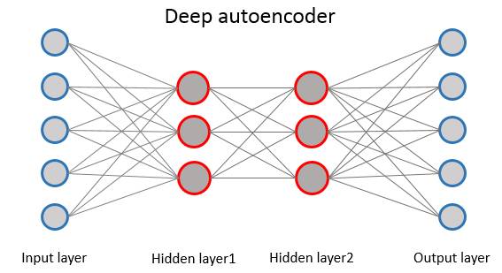
Figure 12. Deep Autoencoder Structure Diagram
Optimization Methods for Deep Networks
Previously, some common deep learning models were introduced. How are these models optimized? This section will introduce some commonly used optimization methods for deep networks.
SGD:
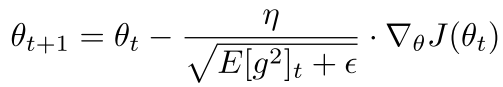
SGD (Stochastic Gradient Descent) is one of the most commonly used optimization methods in machine learning. The working principle of SGD is gradient descent, which adjusts parameters in the direction of the parameter gradient with a certain step size (learning rate), but in SGD, parameters are updated once for a randomly selected sample through gradient descent. When applying SGD in practice, there are several parameters that can be adjusted, mainly including learning rate, weight decay coefficient, momentum, and learning rate decay coefficient. By adjusting these parameters, the model can converge at a faster rate and be less prone to overfitting. The parameter update process of SGD is as follows:
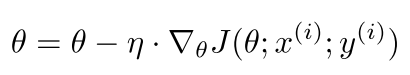
Where θ represents the parameters, η represents the learning rate, and J(θ) represents the optimization objective function, with the gradient of J(θ) with respect to θ calculated on the randomly selected sample  . The advantage of SGD is that it generally achieves good optimization results. However, the parameters (learning rate) of SGD are difficult to adjust, it converges slowly, and it is prone to local optima, potentially getting stuck at saddle points.
Adagrad:
The optimization process of Adagrad is also based on gradients. This optimization method can adaptively adjust different learning rates for each parameter, using a larger learning rate for sparse features and a smaller learning rate for non-sparse features. This adaptive process is achieved by normalizing the current learning rate using accumulated gradients, with the optimization parameter process as follows:
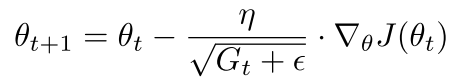
Where  represents the sum of the squares of the gradients of parameter θ over the previous t iterations, and ε is a small value to prevent division by zero errors. The advantage of Adagrad is that it is suitable for handling sparse gradients; however, it still requires a global learning rate η to be set, requires the calculation of the sum of squares of parameter gradients, increasing computational load, and the learning rate decays too quickly.
Adadelta:
Adadelta is an extension of the Adagrad method. As previously mentioned, in Adagrad, the accumulated gradients grow too quickly and lead to rapid decay of the learning rate. The emergence of Adadelta aims to solve this problem. The specific implementation method involves opening a window on the previous parameter sequence, only accumulating the gradients of parameters within that window, and replacing the sum of squares in Adagrad with the mean square. Its parameter update process is as follows:
Where  represents the mean of the squared gradients within the window. Adadelta has the advantage of an adaptive learning rate, with a fast optimization speed, but noticeable fluctuations may occur in the later stages of training.
RMSprop:
The RMSprop optimization method can essentially be seen as a special case of Adadelta. By replacing the 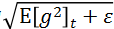 part in Adadelta with the root mean square (RMS) of g, it becomes RMSprop, with parameter updates as follows:

Where  represents the RMS of g. RMSprop’s effect is between Adagrad and Adadelta, making it suitable for non-stationary objectives, but it still relies on a global learning rate parameter.
Adam:
Adam (Adaptive Moment Estimation) is also a method for adaptive parameter learning rates, primarily based on the first and second moments of the gradient to adjust each parameter’s learning rate. The specific parameter update method is as follows:
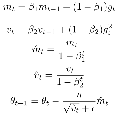
Where  approximates the first moment of the gradient and
  approximates the second moment of the gradient. The corrections ensure that
  approximates an unbiased estimate of the moment. Essentially, Adam is RMSprop with momentum added, making it suitable for handling sparse features and non-stationary target data.
Adamax:
Adamax is a variant of Adam that makes some changes to the learning rate limits, using accumulated gradients and the maximum value from the previous gradient to normalize the learning rate. This limitation is computationally simpler.
Nadam:
Nadam is also a variant of Adam, differing in that it includes a Nesterov momentum term. Generally, Nadam performs better than RMSprop and Adam, but it is more complex computationally.
Common Techniques in Deep Networks
In practical applications, deep learning models are prone to overfitting when the data volume is not large enough. Therefore, techniques and tricks are needed to control the training process, reducing or even preventing severe overfitting. What similar commonly used techniques are there? Next, we will introduce some useful techniques for further optimizing model training.
BP Algorithm:
The BP (Backpropagation) algorithm is merely a method for training neural network models, primarily using the chain rule to compute the derivatives of the objective function concerning parameters, with the derivation process passing backward from the output layer to the input layer. Based on the derived derivatives, the parameters are updated using the optimization algorithms introduced in the previous section, thus optimizing the model. During the application of the BP algorithm to optimize the model, issues such as gradient vanishing, falling into local optima, and gradient instability often arise. These problems can lead to slow convergence and reduced generalization ability of the model. Of course, the occurrence of these problems is also somewhat related to the choice of activation functions in the model, so choosing the activation function reasonably can mitigate these issues to some extent. Currently, commonly used activation functions include sigmoid, tanh, ReLu, PReLu, RReLU, ELU, softmax, etc. Choosing the activation function based on the specific problem is beneficial for the efficient execution of the BP algorithm.
Dropout:
As mentioned earlier, deep learning models are prone to overfitting, mainly due to their complexity and the large number of parameters. When the sample size is not large enough, it is difficult to ensure the model’s generalization ability. Therefore, a method to prevent overfitting called dropout has been proposed, which randomly deactivates some neurons during training to reduce model complexity without affecting the execution of BP. The specific execution process of dropout is illustrated in Figure 13. By comparing the classification performance of the same network before and after using dropout, it has been found that using dropout leads to better prediction results on datasets such as MNIST, CIFAR-10, CIFAR-100, ImageNet, TIMIT, etc.
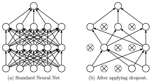
Figure 13. Dropout Process Diagram (Nitish Srivastava et al. 2014)
Batch Normalization:
One significant issue during the training of deep learning networks is that the distribution of data flowing through each layer changes with variations in parameters, a phenomenon known as internal covariate shift. This phenomenon can lead to very slow model training and high requirements for parameter initialization. The emergence of Batch Normalization largely addresses this issue, as it adds a normalization layer directly to the input of each layer, normalizing the input before passing it to the activation function. After processing with Batch Normalization, larger learning rates can be used, thus speeding up training and lowering initialization requirements. The process of training deep networks with Batch Normalization is illustrated in Figure 14. Sergey Ioffe et al. found through experiments that networks with Batch Normalization performed better on the ImageNet dataset.
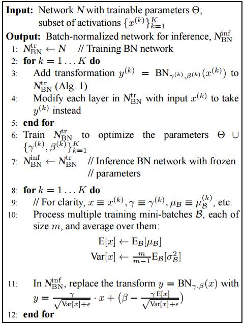
Figure 14. Training Process of Networks with Batch Normalization (Sergey Ioffe et al. 2015)
Early Stopping:
Early stopping is also a technique used in practical applications of deep learning models to prevent overfitting. This technique mainly controls the number of training epochs to prevent overfitting, automatically stopping training when the validation loss no longer decreases. In fact, early stopping can be applied to many machine learning problems, such as non-parametric regression, boosting, etc. Additionally, early stopping can be viewed as a form of regularization.
Regularization:
The regularization mentioned here refers specifically to techniques such as L1 and L2 regularization for controlling weights, excluding previous techniques like Dropout and early stopping. Adding L1 or L2 regularization terms to the network’s weight parameters is a commonly used method to prevent overfitting. L1/L2 regularization methods are widely used in machine learning, and will not be elaborated on further here.
Common Platforms and Frameworks for Deep Learning
Due to the complexity of deep learning models, certain requirements are placed on machine hardware and platforms. A good application platform can significantly enhance the efficiency of model training. So, what popular and useful platforms and frameworks exist for deep learning? Below are some commonly used deep learning platforms along with their pros and cons.
Caffe:
Caffe is a machine learning library developed and maintained by the Visual and Learning Center at the University of California, Berkeley, in 2013. It has excellent implementations for convolutional neural networks (http://caffe.berkeleyvision.org). Caffe is developed based on C/C++, so its computational speed is relatively fast. However, Caffe is not well suited for processing text or sequential data, meaning it has significant limitations in RNN applications. Its pros and cons can be summarized as follows:
Pros: Suitable for image processing; stable version, relatively fast computation speed.
Cons: Not suitable for RNN applications; non-extensible; inconvenient for use in large networks; C/C++ programming difficulty; not updated frequently.
Theano/Tensorflow:
Theano and Tensorflow are both lower-level machine learning libraries and are both symbolic computation frameworks. They are suitable for applications based on convolutional neural networks, recurrent neural networks, and Bayesian networks, providing Python interfaces, with Tensorflow also offering a C++ interface. Theano was developed and maintained by the LISA lab at the Montreal Institute of Technology in 2008 (http://deeplearning.net/software/theano/), making it very suitable for numerical computation optimization and supporting automatic calculation of function gradients, but it does not support multi-GPU applications. Tensorflow was developed by the Google Brain team, is now open-source, and is maintained by the Google Brain team and numerous users (https://www.tensorflow.org).
Tensorflow makes the design of neural network models very easy by numerically computing tensors through pre-defined data flow graphs. Compared to Theano, Tensorflow supports distributed computing and multi-GPU applications. Currently, Tensorflow is the most widely used library for implementing deep learning models.
Keras:
Keras is a high-level deep learning library based on Theano and Tensorflow (https://keras.io/). It was developed by Google software engineer Francois Chollet and is maintained by users after being open-sourced. Keras has a very intuitive API, making it very simple to use; generally, only a few lines of code are needed to build a neural network model. Currently, Keras has released version 2.0, supporting users in customizing network layers from the ground up, greatly addressing the lack of flexibility in previous versions.
Torch/PyTorch:
Torch is a computing framework developed in the Lua language (http://torch.ch/), which supports convolutional neural networks very well. In Torch, networks are defined in a layer-wise manner, which means it does not support the extension of new layer types, but defining new layers is relatively easy. Torch runs on LuaJIT, which is fast; however, Lua is not a mainstream programming language. Additionally, it is worth noting that Facebook announced the Python API for Torch in January 2017, which is the source code for PyTorch. PyTorch supports dynamic computation graphs, making it convenient for users to handle variable-length inputs and outputs. The Python-based library significantly increases the integration flexibility of Torch.
Lasagne:
Lasagne is a computing framework based on Theano (http://lasagne.readthedocs.io/en/latest/index.html). Its level of encapsulation is not as high as Keras, but it provides smaller interfaces, making the code relatively simple compared to the underlying Theano/Tensorflow. This semi-encapsulated feature of Lasagne balances ease of use and customization flexibility.
DL4J:
DL4J (Deeplearning4j) is a deep learning library based on Java (https://deeplearning4j.org/). It was released and open-sourced by Skymind in 2014, and its included deep learning library is an open-source library for commercial applications. Since it is based on Java, it can be integrated with big data processing platforms like Hadoop and Spark. DL4J relies on ND4J for basic linear algebra operations, providing fast computation speed, and it can be automated for parallel processing, making it very suitable for quickly solving practical problems.
MXNet:
MXNet is a deep learning library developed in multiple languages and providing interfaces in various languages (http://mxnet.io/). Supported languages include Python, R, C++, Julia, Matlab, etc., and it provides interfaces in C++, Python, Julia, Matlab, JavaScript, R, etc. MXNet is a fast and flexible learning library developed and maintained by Pedro Domingos and his research team at the University of Washington. Currently, MXNet has been adopted by Amazon Web Services.
CNTK:
CNTK is Microsoft’s open-source deep learning framework (http://cntk.ai), developed based on C++ but providing Python interfaces. CNTK’s features include simple deployment and fast computation speed; however, it does not support ARM architecture. CNTK’s learning library includes feedforward DNNs, convolutional neural networks, and recurrent neural networks.
Neon:
Neon is a deep learning library developed by Nervana (http://neon.nervanasys.com/docs/latest/). This library supports applications like convolutional neural networks, recurrent neural networks, LSTM, and autoencoders, and is currently open-source. Reports indicate that Neon outperforms Caffe, Torch, and Tensorflow in certain tests.
Examples of Deep Learning Networks
Through the previous introduction, readers should have a detailed understanding of deep learning. So how are deep learning networks actually designed in practical applications? This section introduces several deep learning networks with very good application results, from which we can appreciate some design techniques for neural networks.
LeNet:
LeNet is one of the earliest proposed convolutional neural networks by Yann LeCun et al., which has been mentioned when introducing CNNs (Figure 7). The LeNet network consists of 7 layers (excluding the input layer), namely C1, S2, C3, S4, C5, F6, and OUTPUT layers, where C1 and C3 are convolution layers, S2 and S4 are downsampling layers, and C5 and F6 are fully connected layers. The input to this network is 32 x 32 images, with C1 containing 6 feature maps, C3 containing 16 feature maps, and the number of neurons in the two fully connected layers being 120 and 84, respectively. The final output layer contains 10 neurons corresponding to ten categories. This network requires optimization of about 12,000 parameters during training and performs far better than traditional machine learning methods on handwritten digit recognition tasks (MNIST dataset). The proposal of this network provides a model for applying convolutional neural networks, which involves alternating convolutional layers with sampling layers (later pooling layers), ultimately connecting to fully connected layers. Practice has proven that this network structure performs well in many tasks.
AlexNet:
AlexNet is the convolutional neural network used by Alex and Hinton in the ILSVRC2012 competition, marking the beginning of deeper CNN applications on large datasets, with many subsequent applications developed based on this network. AlexNet consists of 5 convolutional layers and 3 fully connected layers, with pooling processes added after the 1st, 2nd, and 5th convolutional layers (Figure 15). The number of neurons in each layer is 253,440, 186,624, 64,896, 64,896, 43,264, 4,096, 4,096, and 1,000, totaling approximately 60 million parameters. The training set for this network consists of 1.4 million high-resolution images from ImageNet, with 50,000 for validation and 150,000 for testing. During the training process, ReLu was used as the activation function, and data augmentation techniques such as horizontal flipping were employed. To prevent overfitting, dropout techniques were also used, and the network was optimized using batch gradient descent with momentum and weight decay. The entire training process lasted 5-6 days on two GTX 580 GPUs. Ultimately, this network achieved the best results in the ILSVRC2012 competition, outperforming other methods significantly.
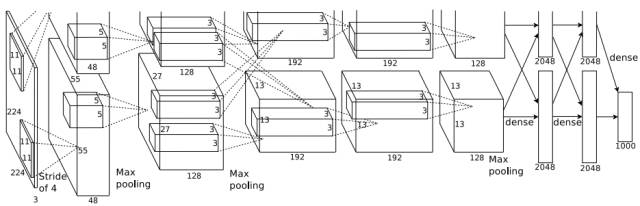
Figure 15. Structure of AlexNet (Alex Krizhevsky et al. 2012)
ZF Net:
ZF Net is a network proposed by Zeiler and Fergus in the ILSVRC2013 competition based on AlexNet. In fact, this network only made some modifications and adjustments to AlexNet, so the structural differences between the two are minimal (Figure 16). The main changes include using smaller convolution kernels in the first convolution layer of ZF Net and reducing the convolution stride to half of the original, which retains more image feature information in the first two layers. The final performance of ZF Net surpassed that of AlexNet, reducing the error rate by 1.7 percentage points. Additionally, the authors of ZF Net proposed a method for visualizing convolutional layer features.
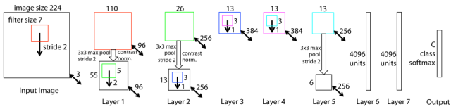
Figure 16. Structure of ZF Net (Matthew D. Zeiler et al. 2013)
VGG Net:
VGG Net is a convolutional neural network model that performed exceptionally well in the ILSVRC2014 competition, characterized by small convolution kernels and deeper convolution layers. This network has a total of 19 layers, including 16 convolutional layers and 3 fully connected layers, with all convolution kernels sized at 3, stacking multiple convolution layers and inserting pooling layers (Figure 17; E). Compared to ZF Net, this network reduced the classification error rate by 9%, significantly improving classification performance. The emergence of VGG Net is significant as it provides an efficient direction for designing and utilizing CNNs, namely, simpler and deeper layers are more conducive to exploring deep features.
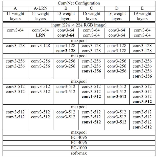
Figure 17. Structure of VGG Net (Karen Simonyan et al. 2014)
GoogLeNet:
GoogLeNet is another convolutional neural network model that appeared in the ILSVRC2014 competition, achieving the best performance in this competition. The depth of GoogLeNet is greater than that of VGG Net, with a total of 22 layers, including 21 convolutional layers and 1 softmax output layer (Figure 18). Notably, this network employs multiple (9) Inception (network in network) modules, meaning that the network does not simply stack layers sequentially but has many parallel connections. Additionally, no fully connected layers are used at the end of the model. The use of Inception modules allows for the collection of more feature information, and the removal of fully connected layers significantly reduces the number of parameters, thereby lowering the potential for overfitting. The final classification results of GoogLeNet improved by 0.6% compared to VGG Net. The significance of GoogLeNet lies in its proposal of a new method for parallel connections between layers, which has provided significant inspiration for future CNN network structure designs.
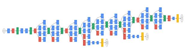
Figure 18. Topology of GoogLeNet (Christian Szegedy et al. 2015)
ResNet:
ResNet is the champion model of the ILSVRC2015 competition, proposed by researchers at Microsoft Research Asia. This network has a depth of 152 layers, including 151 convolution layers and 1 softmax output layer, with residual connections added every two layers (Figure 19). This network model reduces the classification error rate to 3.6%, and its significance lies in proposing a new network structure, namely the residual neural network. The introduction of residual neural networks has addressed the problem of training deep networks to some extent, providing a very good direction for future applications.
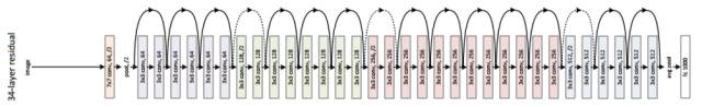
Figure 19. Topology of ResNet (Kaiming He et al. 2015)
Applications of Deep Learning
Computer Vision:
Computer vision is one of the hottest fields for deep learning applications. The previously mentioned network structures are all applied to image classification problems in computer vision, where CNN models are generally chosen to solve such problems. However, there are many other issues in the field of computer vision where simply applying CNN models may not yield good results, such as image captioning, image generation, etc., which require further design of models tailored to specific types of problems.
Currently, the most popular cutting-edge research questions in the field of computer vision include:
-
Image classification, separating different types of images, similar to the tasks in the ILSVRC competition;
-
Image detection, framing different objects in an image;
-
Image segmentation, delineating the boundaries of different objects in an image;
-
Image captioning, describing an image with text;
-
Image generation, generating images based on text descriptions;
-
Video prediction, predicting how objects will move in future frames.
Speech Recognition:
The goal of speech recognition is to convert audio information into text, which is fundamental to human-computer interaction. For this task, traditional solutions generally rely on sequential models to model speech sequences, such as hidden Markov models and Gaussian mixture models, which have relatively high word recognition error rates. The speech recognition process generally involves two aspects: speech feature extraction and acoustic modeling. Researchers have found that using CNNs for speech feature extraction can significantly reduce (by 6%-10%) word recognition error rates (Ossama Abdel-Hamid et al. 2014), and using CNNs for acoustic modeling also demonstrates stronger adaptability. Subsequently, researchers discovered that deeper convolutional neural networks yield better performance, and combining CNN, RNN, and LSTM during the decoding search phase further improves the accuracy of speech recognition. Currently, the IBM Watson Research Center reports that combining ResNet with multiple LSTMs reduces the word error rate in speech recognition to 5.5%. In fact, companies like Apple, Microsoft, and iFlytek employ the latest technologies in their speech recognition systems.
Natural Language Processing:
Natural language processing encompasses various specific applications, mainly including:
-
Part-of-speech tagging, annotating the part of speech for each word in a given sentence;
-
Syntactic analysis, analyzing the grammar of sentence text;
-
Text classification, categorizing content into similar or thematically related texts;
-
Automatic Q&A, a form of human-computer interaction where the human provides a question and the machine responds with an answer;
-
Machine translation, translating between different languages;
-
Automatic summarization, automatically generating a summary of a document.
Currently, deep learning networks have been widely applied to the above tasks. As early as 2014, Nal Kalchbrenner et al. used a dynamic convolutional neural network for sentence modeling (Nal Kalchbrenner et al. 2014), Baotian Hu et al. utilized CNNs to address semantic matching problems, and Chenxi Zhu et al. employed bidirectional LSTM models for text matching issues. Notably, in 2014, a best paper at ACL introduced neural network models into the machine translation process, leading to a surge of deep learning models addressing machine translation issues, significantly improving translation accuracy.
Recommendation Systems:
Recommendation systems are a type of system that pushes information that users may be interested in based on their historical data. The application of deep learning in recommendation systems mainly includes music recommendations, movie recommendations, advertising placements, and news pushes, etc. For example, Balazs Hidasi et al. proposed an RNN-based recommendation system that effectively addresses the problem of traditional recommendation systems being limited to short-term session recommendations; in 2014, Google achieved good results in music ranking using a network similar to MLP; Spotify utilized a typical CNN model for music recommendations.
Extensions of Deep Learning
The rapid development of deep learning has not only made it stand out in many practical applications but has also stimulated the development of many applications or machine learning paradigms that can be easily implemented using deep learning. The impact of deep learning in the field of artificial intelligence is widely recognized; however, relying solely on deep learning cannot sustain the rapid development of artificial intelligence. Therefore, new machine learning methods and network structures have been proposed, and this section focuses on introducing several recently popular learning methods.
Transfer Learning:
Transfer learning refers to utilizing the parameters of a pre-trained model to assist in training a model that needs to be trained. When deep learning networks are relatively deep, training models can become complex and time-consuming. Transfer learning allows the use of previously trained deep network parameters to guide the training of one’s model, thus improving the efficiency of training large networks.
As illustrated in Figure 20, Tasks A, B, and C are three different tasks, but their data has certain correlations, allowing them to share the earlier layers of the network. In other words, the parameters of the earlier layers trained in Task A can guide the training of Tasks B and C. A typical example of transfer learning is the work done by Google DeepMind, where they trained a network model to play three games: Pong, Labyrinth, and Atari, and then used the network trained on one game to play the other two, achieving excellent results. Currently, applications of transfer learning based on deep learning have become very widespread, such as using a mixed model of RBM and CNN for image classification, which has achieved high classification accuracy on the Pascal VOC2007 and Caltech101 datasets.
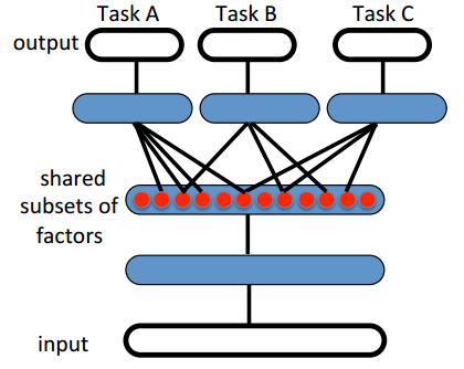
Figure 20. Transfer Learning Diagram (Yoshua Bengio et al. 2014)
Reinforcement Learning:
Reinforcement learning is an important branch of machine learning, with the main idea being that goals act according to changes in the environment to maximize expected benefits. A reinforcement learning model generally includes basic components such as environment, agent, actions, and feedback. Reinforcement learning models are suitable for controlling physical systems (e.g., drones), interacting with users (e.g., optimizing user experience), solving logical problems, learning sequential algorithms, and playing games. A typical example of reinforcement learning is AlphaGo, developed by DeepMind, which enhances its move accuracy by continuously playing against itself. Additionally, there is a learning framework that combines reinforcement learning and deep learning called DQN, which has been applied extensively in natural language processing, such as learning dialogue strategies and information retrieval.
Generative Adversarial Networks:
Generative Adversarial Networks (GANs) were first proposed by Ian Goodfellow et al. in 2014, with the main idea involving two models, G and D. G is responsible for learning the distribution of generated data, while D is responsible for discerning whether the data comes from the real distribution. G’s goal is to generate data that can fool D, while D’s goal is to distinguish G’s generated data. This adversarial process, through iterative training, ultimately yields a generative model for the data G. GANs have seen a surge in research over the past two years, with various variants emerging, such as DCGAN based on CNNs, GANs based on LSTMs (Fang Zhao et al. 2016), GANs based on autoencoders (Alireza Makhzani et al. 2015), and C-RNN-GANs based on RNNs (Olof Mogren et al. 2016). These different variants of GAN models have been widely applied in various fields, including image restoration, super-resolution, de-occlusion, semantic analysis, object detection, and video prediction.
Learning Resources
At the end of the article, we list some learning resources related to deep learning, hoping to be helpful to readers.
GitHub Resources:
-
Resources related to deep learning, including papers, models, books, courses, etc. https://github.com/endymecy/awesome-deeplearning-resources
-
Papers related to adversarial networks: https://github.com/zhangqianhui/AdversarialNetsPapers
-
Deep Learning book edited by Ian Goodfellow et al.: https://github.com/HFTrader/DeepLearningBook
-
Deep learning tutorial provided by the LISA lab: https://github.com/lisa-lab/DeepLearningTutorials
-
Code for Udacity’s deep learning course: https://github.com/udacity/deep-learning
-
Another deep learning resource repository: https://github.com/chasingbob/deep-learning-resources
-
Another comprehensive awesome deep learning resource repository: https://github.com/ChristosChristofidis/awesome-deep-learning
-
A very comprehensive collection of public datasets: https://github.com/XuanHeIIIS/awesome-public-datasets
Online Courses:
-
Stanford’s CS231n by Fei-Fei Li: http://cs231n.github.io
-
Stanford’s CS224d course on NLP by Richard Socher: http://cs224d.stanford.edu/
-
Berkeley’s deep reinforcement learning course CS294 by Sergey Levine et al.: http://rll.berkeley.edu/deeprlcourse/
-
Machine learning course by Nando de Freitas at Oxford: https://www.cs.ox.ac.uk/people/nando.defreitas/machinelearning/
-
Deep learning course by LeCun: http://cilvr.cs.nyu.edu/doku.php?id=courses:deeplearning2014:start
-
Hinton’s neural network course: https://www.coursera.org/learn/neural-networks
-
A teaching video on neural networks: https://www.youtube.com/playlist?list=PL6Xpj9I5qXYEcOhn7TqghAJ6NAPrNmUBH
Conferences/Journals:
-
Conferences: ICLR, NIPS, ICML, CVPR, ICCV, ECCV, ACL
-
Journals: JMLR, MLJ, Neural Computation, JAIR, Artificial Intelligence
Main References for This Article:
[1]. Ian Goodfellow et al. Deep Learning. 2016
[2]. Yoshua Bengio et al. Representation Learning: A Review and New Perspectives. 2014
[3]. Yann LeCun et al. Gradient-based learning applied to document recognition. 1998
[4]. Alex Krizhevsky et al. ImageNet Classification with Deep Convolutional Neural Networks. 2012
[5]. Matthew D Zeiler et al. Visualizing and Understanding Convolutional Networks. 2013
[6]. Nitish Srivastava et al. Dropout: A Simple Way to Prevent Neural Networks from Overfitting. 2014
[7]. Sergey Ioffe et al. Batch Normalization: Accelerating Deep Network Training by Reducing Internal Covariate Shift. 2015
[8]. 侯一民,周慧琼,王政一. 深度学习在语音识别中的研究进展综述。2016
[9]. 刘树杰,董力,张家俊等. 深度学习在自然语言处理中的应用。2015
[10]. Understanding LSTM Networks. colah’s blog
Author: Xuanyuan (pen name), volunteer at DataPi Research Department, graduate student at Tsinghua University, interested in topics related to machine learning and big data.
【Review of Previous Issues in the “Understanding” Series】:
Exclusive | Understanding Transfer Learning (with Learning Toolkit)
Exclusive | Understanding Big Data Processing Frameworks
Exclusive | Understanding Feature Engineering
Exclusive | Understanding Data Visualization
Exclusive | Understanding Clustering Algorithms
Exclusive | Understanding Association Analysis
Exclusive | Understanding Big Data Computing Frameworks and Platforms
Exclusive | Understanding Optical Character Recognition (OCR)
Exclusive | Understanding Regression Analysis
Exclusive | Understanding Non-relational Databases (NoSQL)
Introduction to DataPi Research Department
The DataPi Research Department was established in early 2017, aiming to create a first-class structured knowledge sharing platform and an active community of data science enthusiasts, dedicated to spreading data thinking, improving data capabilities, exploring data value, and achieving integration of industry, academia, and research!
The logic of the research department lies in structuring knowledge and gaining true knowledge through practice: organizing a structured foundational knowledge network; original hands-on teaching and practical experience articles; forming professional interest communities for交流学习、team practice, and tracking frontiers. Interest groups are the core of the research department, each following the overall knowledge sharing and practical project planning of the research department, while having their own characteristics: Algorithm Model Group: actively participating in competitions like Kaggle, original hands-on teaching series articles; Research and Analysis Group: exploring the beauty of data products through interviews; System Platform Group: tracking cutting-edge technologies in big data & artificial intelligence systems, dialoguing with experts; Natural Language Processing Group: focusing on practice, actively participating in competitions and planning various text analysis projects; Manufacturing Big Data Group: pursuing the dream of an industrial powerhouse, integrating industry, academia, and government to explore data value; Data Visualization Group: merging information with art, exploring the beauty of data, and learning to tell stories through visualization; Web Crawler Group: crawling web information, collaborating with other groups to develop creative projects.
Click the “Read Original” at the end of the article to register for the DataPi Research Department Volunteer, there is always a group that suits you~
Notice for Reprinting
If you need to reprint the article, please do the following: 1. Indicate at the beginning of the text: Reprinted from DataPi THU (ID: DatapiTHU);2. Attach the DataPi QR code at the end of the article.
To apply for reprinting, please send an email to [email protected]

The bottom menu of the official account has surprises!
For enterprises and individuals joining the organization, please check the “Federation”
For exciting past content, please check the “Search in Account”
For joining volunteers or contacting us, please check the “About Us”

Click “Read Original” to join the organization~