

Source: Original article by CSDN blogger “Fate_fjh”.
The traditional CNN network can only provide the LABEL of an image, but in many cases, it is necessary to segment the identified objects to achieve end to end recognition. This is where FCN comes in, providing a very important solution for object segmentation, with the core being convolution and deconvolution. Therefore, we will explain convolution and deconvolution in detail here.
For 1D convolution, the formulas (discrete) and calculation process (continuous) are as follows. It is important to remember that one of the functions (the original function or the convolution function) must be flipped 180 degrees before convolution.
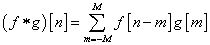
Figure 1
For discrete convolution, the size of f is n1, the size of g is n2, and the size after convolution is n1+n2-1.

Figure 2
Similarly, during convolution, the convolution kernel must be rotated 180 degrees, and the center of the convolution kernel must be aligned with the pixel of the image being calculated. The output structure is a new pixel value centered on the aligned pixel. An example of the calculation is as follows:
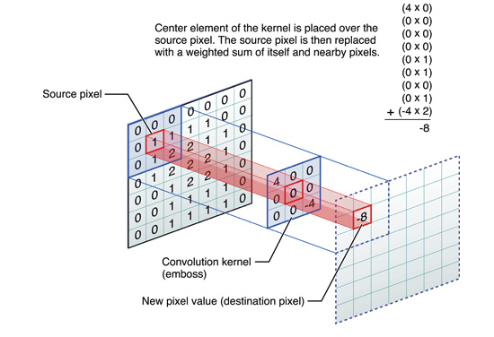
Figure 3
This calculates the convolution pixel value for the top left corner (i.e., the first row and first column) pixel.
Here is a more intuitive example: from left to right, the original pixel changes from 1 to -8 after convolution.

Figure 4
In signal processing, reversing 180 degrees is called convolution, while direct sliding calculation is called autocorrelation. Most deep learning frameworks do not perform the 180-degree reversal operation.
By sliding the convolution kernel, we can obtain the convolution result of the entire image.
Figure 5
At this point, we can roughly understand image convolution. However, we can see that after image convolution, the size of the new image is the same as or smaller than the original. The image size remains the same after the calculation in Figure 2, while the image in Figure 5 becomes smaller because not all pixels were used for convolution calculation. But didn’t the 1D convolution result get larger? Let’s explain that below.
In MATLAB, the calculation of 2D convolution is divided into three categories: full, same, and valid. (Reference: https://cn.mathworks.com/help/matlab/ref/conv2.html?requestedDomain=www.mathworks.com)
The convolution corresponding to Figure 2 is called same, while that corresponding to Figure 5 is valid. So what is full? See the following figure.

Figure 6
Figure Source: https://github.com/vdumoulin/conv_arithmetic
In Figure 6, blue is the original image, white is the corresponding padding added for convolution (usually all zeros), and green is the image after convolution. The sliding of the convolution in Figure 6 starts from the overlap of the bottom right corner of the convolution kernel with the top left corner of the image, with a sliding step of 1. The center element of the convolution kernel corresponds to the pixel point of the image after convolution. We can see that the image after convolution is 4X4, which is larger than the original 2X2 image. We remember that the size of 1D convolution is n1+n2-1. Here, the original image is 2X2, and the convolution kernel is 3X3, resulting in a 4X4 output, which corresponds exactly to the one-dimensional case. This is actually the complete convolution calculation; other smaller convolution results have skipped some pixel convolutions. Below is an explanation of the extra parts after image convolution according to WIKI: Kernel convolution usually requires values from pixels outside of the image boundaries. There are a variety of methods for handling image edges. This means that the extra parts can be handled differently based on the actual situation. (In fact, the full convolution here is what will be discussed later as deconvolution.)
Here, we can summarize the formulas for calculating the size of the image after full, same, and valid convolutions:
-
full: Sliding step is 1, image size is N1xN1, convolution kernel size is N2xN2, the size after convolution is: N1+N2-1 x N1+N2-1. As shown in Figure 6, with a sliding step of 1, the image size is 2×2, the convolution kernel size is 3×3, and the size after convolution is 4×4.
-
same: Sliding step is 1, image size is N1xN1, convolution kernel size is N2xN2, the size after convolution is: N1xN1.
-
valid: Sliding step is S, image size is N1xN1, convolution kernel size is N2xN2, the size after convolution is: (N1-N2)/S+1 x (N1-N2)/S+1. As shown in Figure 5, with a sliding step of 1, the image size is 5×5, the convolution kernel size is 3×3, and the size after convolution is 3×3.
The deconvolution mentioned here is very different from the deconvolution calculation in 1D signal processing. The authors of FCN refer to it as backward convolution, and some people call it the Deconvolution layer, which is a very unfortunate name and should rather be called a transposed convolutional layer. We know that in CNN, there are con layers and pool layers. The con layer performs convolution on images to extract features, while the pool layer reduces the image size by half to filter important features. For classic image recognition CNN networks, such as IMAGENET, the final output is 1X1X1000, where 1000 is the number of categories, and 1×1 is the result obtained. The authors of FCN or later researchers studying end to end recognition use deconvolution on the final 1×1 result (in fact, the final output of the FCN authors is not 1X1, but 1/32 of the image size, but this does not affect the use of deconvolution).
The deconvolution of the image here is similar in principle to the full convolution in Figure 6, using this method of deconvolution allows the image to enlarge. The method used by the FCN authors is a variant of the deconvolution mentioned here, which allows for the corresponding pixel values to be obtained, enabling the image to achieve end to end recognition.
Figure 7
Figure Source: https://github.com/vdumoulin/conv_arithmetic
Here is another method of deconvolution. Suppose the original image is 3X3, we first use upsampling to make the image 7X7, and we can see that there are many blank pixels added to the image. Then, we use a 3X3 convolution kernel to perform valid convolution with a sliding step of 1 on the image, resulting in a 5X5 image. What we know is that upsampling enlarges the image, and deconvolution fills in the image content, enriching the image content. This is also one method for CNN to output end to end results. The Korean author Hyeonwoo Noh uses a VGG16 layer CNN network followed by a symmetrical 16-layer deconvolution and upsampling network to achieve end to end output. The effects of different layers of upsampling and deconvolution are shown in Figure 8.
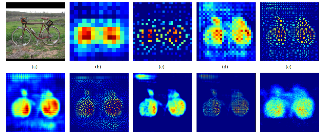
Figure 8
After the above explanations and derivations, we have a basic understanding of convolution. However, the concept of deconvolution on images may still not be well understood. Therefore, let’s explain this process again.
Currently, there are two most commonly used methods of deconvolution, which have been introduced above.
-
Method 1: Full convolution, which can enlarge the original domain.
-
Method 2: Record pooling index, then expand space, and use convolution to fill.
The deconvolution process of the image is as follows:
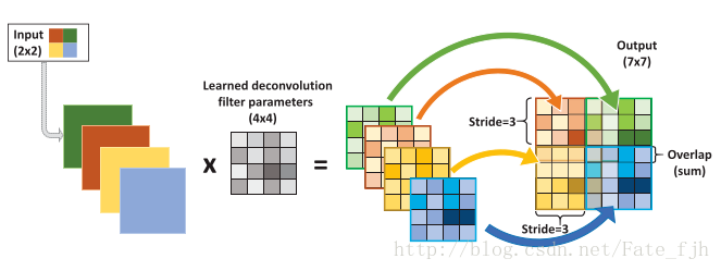
Figure 9
Input: 2×2, convolution kernel: 4×4, sliding step: 3, output: 7×7.
This means that the input is a 2×2 image going through a 4×4 convolution kernel with a sliding step of 3:
-
Each pixel of the input image performs a full convolution. Based on the size of the full convolution, we can know that the size after convolution for each pixel is 1+4-1=4, which means a 4×4 size feature map. Since the input has 4 pixels, there are 4 feature maps of 4×4.
-
These 4 feature maps are fused with a sliding step of 3 (i.e., added together). For example, the red feature map remains in the original input position (top left), the green one remains in the original position (top right), and the sliding step of 3 means that fusion occurs every 3 pixels, with overlapping parts being summed. That is, the output’s first row and fourth column is obtained by adding the first row and fourth column of the red feature map with the first row and first column of the green feature map, and so on.
It can be seen that the size of deconvolution is determined by the size of the convolution kernel and the sliding step. In is the input size, k is the convolution kernel size, s is the sliding step, and out is the output size. The output is calculated as out=(in-1)*s+k. The process in the above figure is (2-1)*3+4=7.
Original link:
https://blog.csdn.net/fate_fjh/article/details/52882134

A popular explanation of the definition and significance of convolution

Disclaimer: This WeChat reposted article is for non-commercial educational and research purposes and does not imply endorsement of its views or confirmation of its content’s authenticity. Copyright belongs to the original author. If there are copyright issues with the reprint, please contact us immediately!