Source: Artificial Intelligence AI Technology


This article is about 2500 words long and is recommended for a 9-minute read.
This article organizes the development history of CNN network structures.

Author丨zzq

Source丨https://zhuanlan.zhihu.com/p/68411179

Introduction to Basic Components of CNN

1. Local Receptive Field

In images, the connections between local pixels are relatively tight, while the connections between distant pixels are relatively weak. Therefore, each neuron does not need to perceive the entire image; it only needs to perceive local information, which can then be integrated at higher levels to obtain global information. The convolution operation is the realization of the local receptive field, and because convolution operations can share weights, it also reduces the number of parameters.

2. Pooling

Pooling reduces the size of the input image, minimizing pixel information while retaining important information, primarily to reduce computational load. It mainly includes max pooling and average pooling.

3. Activation Function

The activation function is used to introduce non-linearity. Common activation functions include sigmoid, tanh, and ReLU; the first two are commonly used in fully connected layers, while ReLU is common in convolutional layers.

4. Fully Connected Layer

The fully connected layer acts as a classifier in the entire convolutional neural network. The outputs from previous layers need to be flattened before entering the fully connected layer.

Classic Network Structures

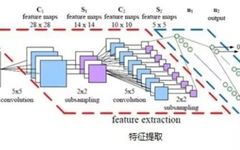
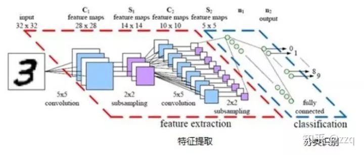
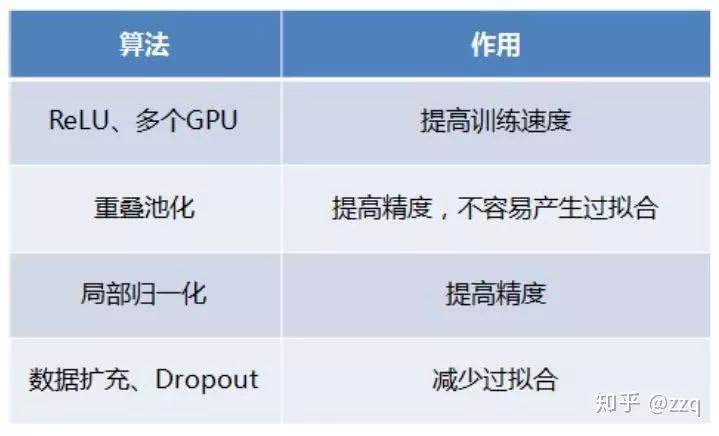
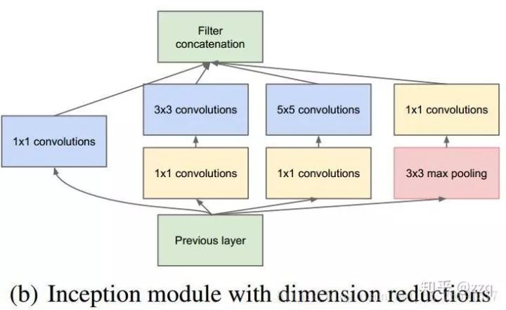
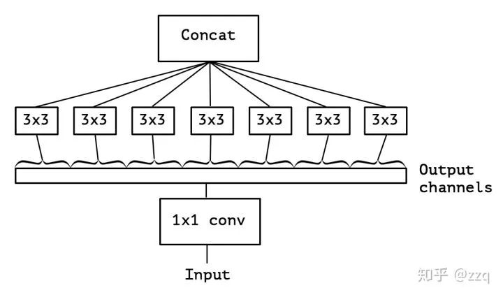
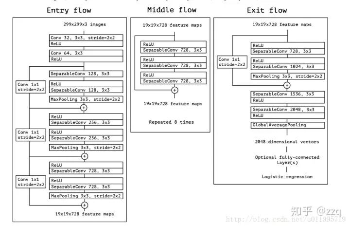
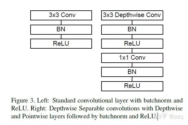
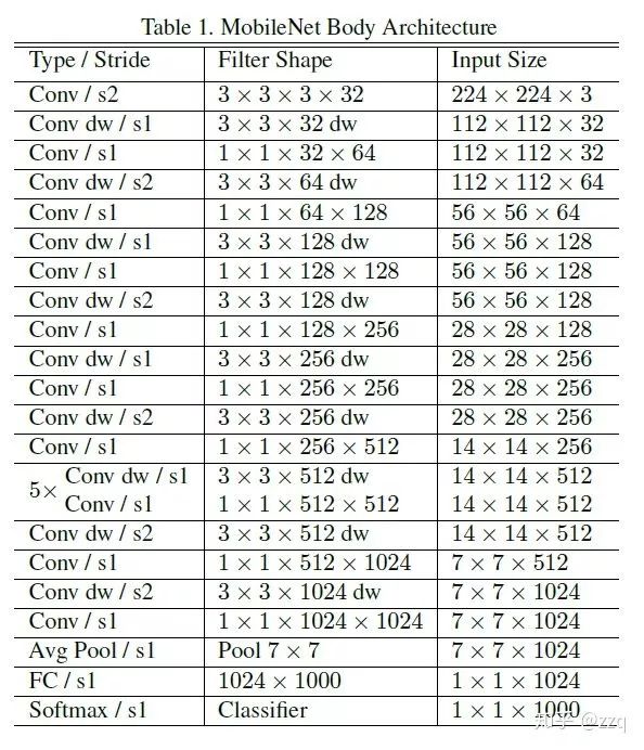
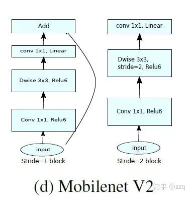
1. LeNet5

Consists of two convolutional layers, two pooling layers, and two fully connected layers. The convolution kernels are all 5×5, with stride=1, and the pooling layer uses max pooling.

2. AlexNet

The model has eight layers (excluding the input layer), including five convolutional layers and three fully connected layers. The last layer uses softmax for classification output.

AlexNet uses ReLU as the activation function; it prevents overfitting using dropout and data augmentation; achieves dual GPU implementation; and employs LRN.

3. VGG

All layers use stacked 3×3 convolution kernels to simulate a larger receptive field, and the network depth is increased. VGG has five segments of convolutions, each followed by a max pooling layer. The number of convolution kernels gradually increases.

Summary: LRN has little effect; deeper networks yield better performance; 1×1 convolutions are also effective but not as good as 3×3.

4. GoogLeNet (Inception v1)

From VGG, we learned that deeper networks yield better performance. However, as models become deeper, the number of parameters increases, making the network more prone to overfitting, requiring more training data; additionally, complex networks mean more computational load and larger model storage, requiring more resources and slower speeds. GoogLeNet was designed to reduce parameters.

GoogLeNet increases network complexity by widening the network, allowing it to choose how to select convolution kernels. This design reduces parameters while improving the network’s adaptability to multiple scales. It uses 1×1 convolutions to increase network complexity without adding parameters.

Inception-v2

On the basis of v1, batch normalization technology is added. In TensorFlow, using BN before the activation function yields better results; the 5×5 convolutions are replaced with two consecutive 3×3 convolutions, making the network deeper with fewer parameters.

Inception-v3

The core idea is to decompose convolution kernels into smaller convolutions, such as decomposing 7×7 into 1×7 and 7×1 convolutions, reducing network parameters while increasing depth.

Inception-v4 Structure

Introduces ResNet to accelerate training and improve performance. However, when the number of filters is too large (>1000), training becomes unstable; an activate scaling factor can be added to alleviate this.

5. Xception

Proposed based on Inception-v3, the basic idea is depthwise separable convolutions, but with differences. The model parameters are slightly reduced, but accuracy is higher. Xception first performs a 1×1 convolution followed by a 3×3 convolution, merging channels before performing spatial convolutions. Depthwise is the opposite, first performing spatial 3×3 convolutions followed by channel 1×1 convolutions. The core idea is to follow the assumption that convolutions should separate channel convolutions from spatial convolutions. MobileNet-v1 uses the depthwise order and adds BN and ReLU. The parameter count of Xception is not much different from that of Inception-v3; it increases network width to improve accuracy, while MobileNet-v1 aims to reduce parameters and improve efficiency.

6. MobileNet Series

V1

Uses depthwise separable convolutions; abandons pooling layers and uses stride=2 convolutions. The number of channels in the standard convolution kernel equals the number of channels in the input feature map; while the depthwise convolution kernel has a channel count of 1; two parameters can control it, ‘a’ for input-output channel count; ‘p’ for image (feature map) resolution.

V2

Three differences compared to v1:

1. Introduced residual structure;

2. Performed 1×1 convolution before dw to increase feature map channel count, which is different from traditional residual blocks;

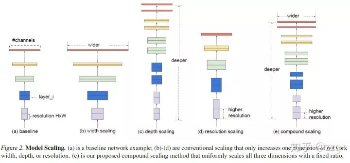
3. After pointwise, ReLU is discarded in favor of a linear activation function to prevent ReLU from damaging features.

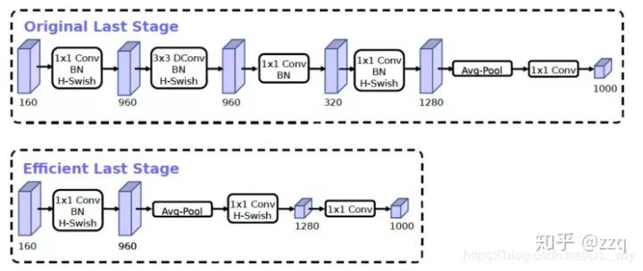
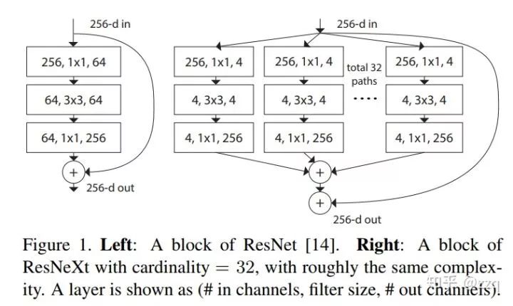
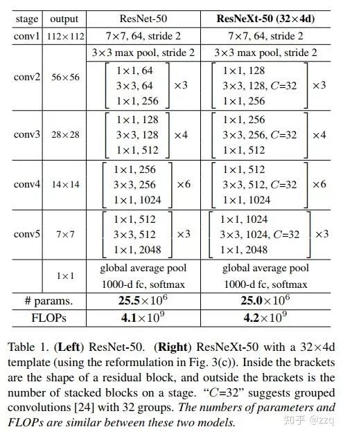
This is because the features extracted by the dw layer are limited by the input channel count; if a traditional residual block is used, compressing the features that dw can extract would yield even fewer features. Therefore, it is better to expand first. However, when using expansion-convolution-compression, after compression, ReLU can damage features, and since the features are already compressed, further passing through ReLU would lose some features, so linear should be used.

V3

Complementary search technology combination: executed module set search by resource-constrained NAS, and NetAdapt executes local search; network structure improvement: moves the last average pooling layer forward and removes the last convolution layer, introducing the h-swish activation function, and modifies the starting filter group.

V3 integrates the depthwise separable convolutions of v1, the linear bottleneck of v2, and the lightweight attention model of SE structure.

7. EffNet

EffNet is an improvement over MobileNet-v1, with the main idea being: decompose the dw layer of MobileNet-1 into two 3×1 and 1×3 dw layers, so that pooling is applied after the first layer, reducing the computational load of the second layer. EffNet is smaller and progresses faster than MobileNet-v1 and ShuffleNet-v1 models.

8. EfficientNet

The research on network design focuses on expanding in depth, width, and resolution, and understanding their interrelationships can achieve higher efficiency and accuracy.

9. ResNet

VGG proved that increasing the depth of the network layers is an effective way to improve accuracy; however, deeper networks are prone to gradient vanishing, leading to poor convergence. Tests show that beyond 20 layers, convergence worsens with increasing depth. ResNet effectively addresses the issue of gradient vanishing (actually alleviating it rather than completely solving it) by adding shortcut connections.

10. ResNeXt

Based on ResNet and Inception’s split+transform+concatenate approach. However, its performance surpasses that of ResNet, Inception, and Inception-ResNet. Group convolution can be used. Generally, there are three ways to enhance network expressiveness:

1. Increase network depth, e.g., from AlexNet to ResNet, but experimental results show that the improvement brought by network depth diminishes;

2. Increase the width of network modules, but increasing width inevitably leads to exponential growth in parameter scale, which is not mainstream in CNN design;

3. Improve CNN network structure design, such as Inception series and ResNeXt. Experiments have found that increasing cardinality, which refers to the number of identical branches in a block, can better enhance model expressiveness.

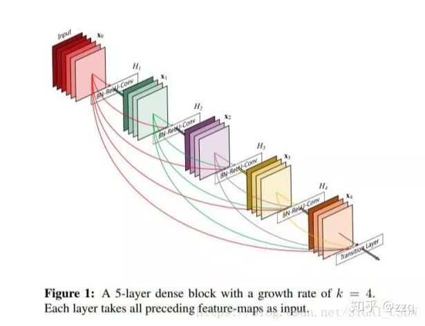
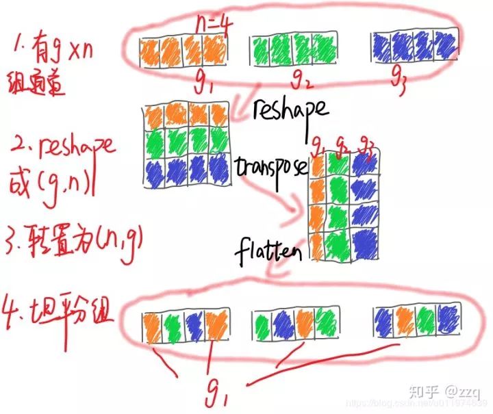
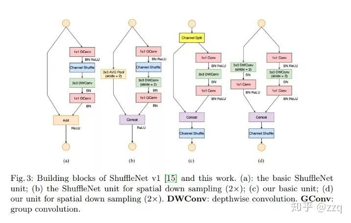
11. DenseNet

DenseNet significantly reduces the number of parameters through feature reuse, while also alleviating the gradient vanishing problem to some extent.

12. SqueezeNet

Proposed the fire-module: squeeze layer + expand layer. The squeeze layer uses 1×1 convolution, while the expand layer uses both 1×1 and 3×3 convolutions, followed by concatenation. SqueezeNet has only 1/50 the parameters of AlexNet, and after compression, it has 1/510, yet its accuracy is comparable to that of AlexNet.

13. ShuffleNet Series

V1

Reduces computational load through grouped convolutions and 1×1 pointwise group convolutions, enriching the information of various channels through channel reorganization. Xception and ResNeXt are inefficient in small network models due to the resource-intensive nature of numerous 1×1 convolutions; thus, pointwise group convolutions were proposed to reduce computational complexity, but using pointwise group convolutions can have side effects. Therefore, channel shuffle was proposed to facilitate information flow. Although dw can reduce computational load and parameter count, on low-power devices, it is less efficient in terms of computation and storage access compared to dense operations. Hence, ShuffleNet aims to use depthwise convolutions at the bottleneck to minimize overhead.

V2

Design criteria for more efficient CNN network structures:

• Maintaining equal input and output channel counts can minimize memory access costs;

• Using too many groups in grouped convolutions increases memory access costs;

• Excessively complex network structures (too many branches and basic units) can reduce network parallelism;

• Element-wise operations also consume resources and should not be overlooked.

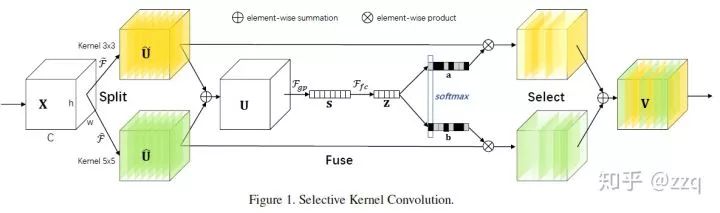
14. SENet

15. SKNet

Copyright Statement: Content sourced from the internet, copyright belongs to the original creator. Unless otherwise indicated, the author and source will be marked. If there is any infringement, please inform us, and we will delete it immediately and apologize!

Editor: Huang Jiyan