
Click on the above “Beginners Learn Vision”, select to add “Star” or “Top”
Important content delivered at the first time
Data and Background
CNN Principles
CNN, also known as Convolutional Neural Networks, is an important branch of deep learning. CNN performs excellently in many fields, with accuracy and speed much higher than traditional computational learning algorithms. Especially in the field of computer vision, CNN is the mainstream model for solving image classification, image retrieval, object detection, and semantic segmentation.
1. Convolution
As shown in Figure 1, regardless of how the X and O are rotated or scaled, the human eye can easily recognize X and O.

Figure 1
However, computers are different; they see an array of pixels, as shown in Figure 2. The task of extracting features from the pixel array is precisely what convolutional neural networks are designed to do.
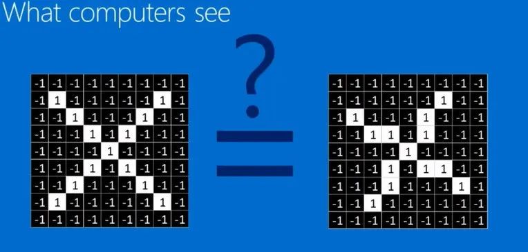
Figure 2
Looking at Figure 3, we find that even if X is rotated, the areas marked by green, orange, and purple boxes are still consistent in both images. To some extent, this is actually the feature of X.

Figure 3
Therefore, these three feature intervals can be extracted to form three convolution kernels, as shown in Figure 4.

Figure 4
Now that we have convolution kernels, how do they perform convolution operations? It’s quite simple, as seen in Figure 5, the convolution kernel slides over the image matrix bit by bit, just like sweeping the floor. Each time it sweeps to a location, a convolution operation can be performed. The calculation method is straightforward; as shown in Figure 5, when the kernel sweeps to the position indicated by the green box, the numbers in the convolution kernel matrix correspond to the numbers in the swept matrix, which are multiplied and summed, and the final value is the feature extracted by the convolution kernel.

Figure 5
All features extracted by the convolution kernels form a matrix with reduced height and width, known as the feature map, as shown in Figure 6. Different convolution kernels can extract different feature maps. Therefore, it can be imagined that if convolution operations are continuously performed, the dimensions of the image matrix will gradually decrease while its depth increases.

Figure 6
2. Pooling
Pooling is actually a process of further refining each feature map. As shown in Figure 7, the original 4X4 feature map becomes a smaller 2*2 matrix after pooling. Pooling methods include max pooling, which takes the maximum value, and average pooling, which takes the average value.

Figure 7
3. Normalization
Here, normalization refers to converting negative values in the matrix to 0, using an activation function called ReLU to perform the operation of turning negative numbers to 0. The ReLU function is essentially max(0, x). This step is also to facilitate calculations.
4. Understanding Convolutional Neural Networks
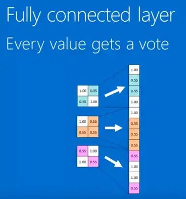
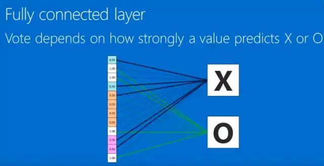
Therefore, convolution, ReLU, and pooling, when repeatedly applied, basically form the framework of convolutional neural networks, as shown in Figure 8. The final feature map is arranged in a row (Figure 8) and connected to the fully connected layer, thus forming our convolutional neural network. It is worth noting that the values arranged in a row have weights, which are obtained through training and backpropagation. By calculating the weights, we can understand the probabilities of different classifications.
 Figure 8
Convolutional Neural Networks
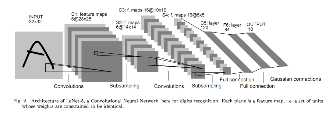
The structure of the LeNet network is shown below, with a total of 7 layers (excluding the input layer), including 2 convolutional layers, 2 pooling layers, and 3 fully connected layers.

In the convolutional layer block, the input height and width decrease layer by layer. The convolutional layers, using a 5*5 kernel, reduce the height and width by 4, while the pooling layers halve the height and width, but the number of channels increases from 1 to 16. The fully connected layers gradually reduce the output count until it becomes the number of categories in the image, which is 10.
The effect of digit recognition is shown in the figure:

Advanced Convolutional Neural Networks
With the development of network structures, researchers initially found that deeper network models with more parameters yield better accuracy. A typical progression includes AlexNet, VGG, InceptionV3, and ResNet. 
1. AlexNet (2012)
In 2012, AlexNet made its debut. The model is named after the first author of the paper, Alex Krizhevsky. AlexNet used an 8-layer convolutional neural network and won the ImageNet 2012 image recognition challenge with a large advantage. It first proved that learned features could surpass hand-designed features, breaking new ground in computer vision research.
 AlexNet and LeNet share similar design philosophies but have significant differences.
Summary:
-
AlexNet has a structure similar to LeNet but uses more convolutional layers and a larger parameter space to fit the large-scale ImageNet dataset. It serves as the dividing line between shallow and deep neural networks.
-
Although it seems that the implementation of AlexNet only adds a few lines of code compared to LeNet, the conceptual shift and the generation of truly excellent experimental results took the academic community many years.
2. VGG-16 (2014)
Building on LeNet, AlexNet added 3 convolutional layers. However, the authors of AlexNet made numerous adjustments to the convolution window sizes, output channel counts, and construction sequences. Although AlexNet indicated that deep convolutional neural networks could achieve outstanding results, it did not provide simple rules to guide future researchers on how to design new networks. VGG, named after the Visual Geometry Group, the laboratory of the paper’s authors, proposed the idea of constructing deep models by repeatedly using simple basic blocks. The structure diagram of VGG is as follows:

The composition pattern of VGG blocks is: consecutive use of several convolutional layers with padding of 1 and a window shape of 3*3, followed by a max pooling layer with a stride of 2 and a window shape of 2*2. The convolutional layers maintain the input height and width, while the pooling layers halve them. We use vgg_block function to implement this basic VGG block, which can specify the number of convolutional layers and input/output channel counts.
For a given receptive field (the local size of the input image related to the output), using stacked small convolution kernels is superior to using large convolution kernels, as it can increase the network depth to ensure the learning of more complex patterns while incurring lower costs (fewer parameters). For example, in VGG, three 3×3 convolution kernels are used instead of a 7×7 convolution kernel, and two 3×3 convolution kernels are used instead of a 5*5 convolution kernel. This approach primarily aims to enhance the depth of the network while maintaining the same receptive field, thereby improving the performance of the neural network to some extent.
VGG: Constructing deep models by repeatedly using simple basic blocks. Block: several identical convolution layers with padding of 1 and a window shape of 3×3, followed by a max pooling layer with a stride of 2 and a window shape of 2×2. The convolution layers maintain the input height and width, while the pooling layers halve them. A comparison of the network diagrams of VGG and AlexNet is shown below:

 Summary: VGG-11 constructs the network by using 5 reusable convolution blocks. Different VGG models can be defined based on the number of convolutional layers and output channel counts in each block.
3. Network in Network (NiN)
LeNet, AlexNet, and VGG: First, fully extract spatial features using modules composed of convolutional layers, and then output classification results using modules composed of fully connected layers. NiN: Chain multiple small networks composed of convolutional layers and “fully connected” layers to construct a deep network. The NiN blocks have an output channel count equal to the number of label categories, and then use global average pooling to average all elements in each channel and directly use it for classification.

1×1 Convolution Kernel Functions
-
Scaling the number of channels: Achieving channel scaling by controlling the number of convolution kernels;
-
Increasing non-linearity. The convolution process of the 1×1 convolution kernel is equivalent to the computation process of a fully connected layer, and it also adds a non-linear activation function, thereby increasing the non-linearity of the network;
-
Computing fewer parameters.
We know that in NiN, the input and output of the convolutional layers are usually four-dimensional arrays (samples, channels, height, width), whereas the input and output of fully connected layers are usually two-dimensional arrays (samples, features). If we want to connect a convolutional layer after a fully connected layer, we need to transform the output of the fully connected layer into four dimensions. Recall that in the multi-input and multi-output channels section, the 1*1 convolution layer can be regarded as a fully connected layer, where each element in the spatial dimensions (height and width) corresponds to samples, and channels correspond to features. Therefore, NiN uses the 1*1 convolution layer to replace the fully connected layer, allowing spatial information to naturally propagate to subsequent layers.
Summary:
-
NiN constructs deep networks by repeatedly using NiN blocks composed of convolutional layers and 1*1 convolution layers that replace fully connected layers.
-
NiN removes the fully connected output layers that are prone to overfitting and replaces them with NiN blocks whose output channel counts equal the number of label categories and global average pooling layers.
-
The design philosophy of NiN has influenced the design of subsequent convolutional neural networks.
4. Networks with Parallel Connections (GoogLeNet)
In the 2014 ImageNet image recognition challenge, a network structure called GoogLeNet shone brightly. Although it pays homage to LeNet in name, it is difficult to see any resemblance to LeNet in its network structure. GoogLeNet absorbed the idea of chaining networks from NiN and made significant improvements on that basis. In the following years, researchers made several improvements to GoogLeNet, and this section will introduce the first version of this model series.
-
Composed of Inception basic blocks.
-
The Inception block is equivalent to a sub-network with 4 parallel lines. It extracts information in parallel through convolution layers and max pooling layers with different window shapes, and uses 1×1 convolution layers to reduce the number of channels, thus lowering model complexity.
-
The customizable hyperparameter is the output channel count of each layer, which we use to control model complexity.
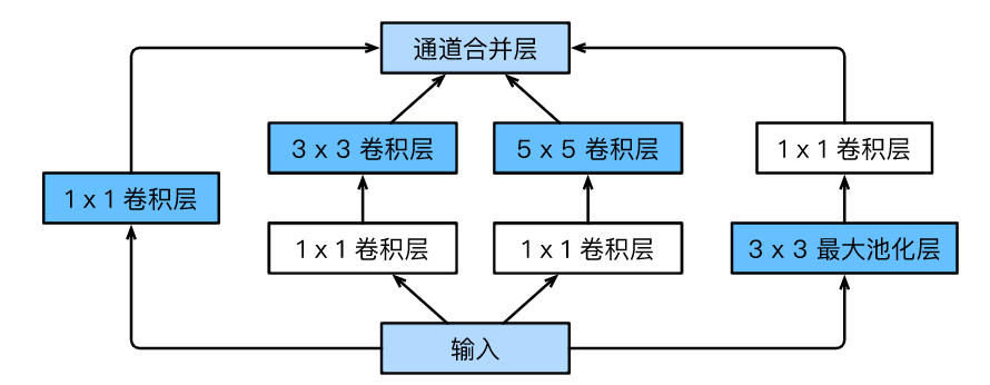 Inception blocks have 4 parallel lines. The first three lines use convolution layers with window sizes of 1*1, 3*3, and 5*5 to extract information at different spatial dimensions, where the middle two lines first perform 1*1 convolutions to reduce the number of input channels to lower model complexity. The fourth line uses a 3*3 max pooling layer followed by a 1*1 convolution layer to change the number of channels. All four lines use appropriate padding to keep the input and output height and width consistent. Finally, we concatenate the outputs of each line along the channel dimension and feed them into the next layer. The customizable hyperparameter in the Inception block is the output channel count of each layer, which we use to control model complexity. Like VGG, GoogLeNet uses 5 modules (blocks) in the main convolution part, with each module using a 3*3 max pooling layer with a stride of 2 to reduce the output height and width.
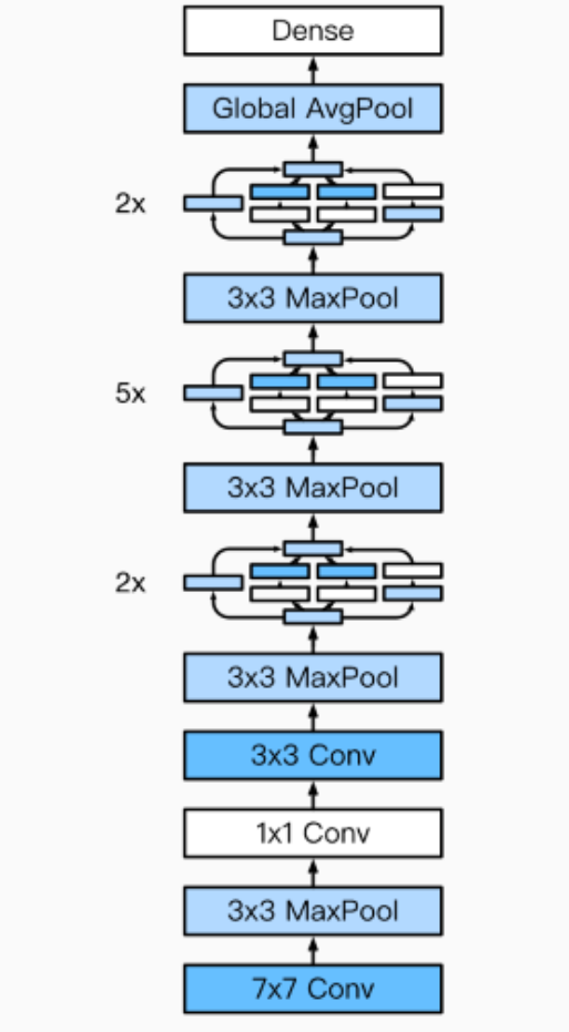
Summary:
-
The Inception block is equivalent to a sub-network with 4 parallel lines. It extracts information in parallel through convolution layers and max pooling layers with different window shapes and uses 1*1 convolution layers to reduce the number of channels, thus lowering model complexity.
-
GoogLeNet strings together multiple finely designed Inception blocks and other layers. The channel count ratios in the Inception blocks are obtained through extensive experimentation on the ImageNet dataset.
-
GoogLeNet and its successors were once among the most efficient models on ImageNet: they often had lower computational complexities for similar test accuracies.
5. Residual Networks (ResNet-50)
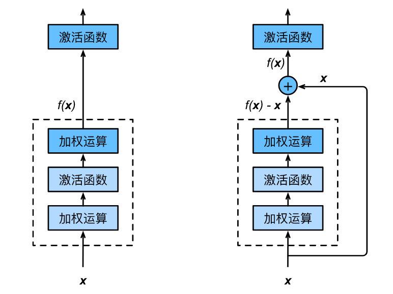
The problem with deep learning: Simply increasing the number of layers in deep CNN networks after reaching a certain depth does not lead to further improvements in classification performance; instead, it can cause the network to converge more slowly and decrease accuracy.
-
Left: f(x)=x;
-
Right: f(x)-x=0 (easy to capture subtle fluctuations in the identity mapping).
The first two layers of ResNet are the same as those in GoogLeNet: a 7*7 convolution layer with an output channel count of 64 and a stride of 2, followed by a 3*3 max pooling layer with a stride of 2. The difference is that ResNet adds batch normalization layers after each convolution layer. The structure of the ResNet-50 network is as follows:

Summary:
-
Residual blocks enable the effective training of deep neural networks through cross-layer data channels.
-
ResNet has profoundly influenced the design of subsequent deep neural networks.
Building Models with Pytorch
import torchtorch.manual_seed(0)torch.backends.cudnn.deterministic= Falsetorch.backends.cudnn.benchmark = Trueimport torchvision.models as modelsimport torchvision.transforms as transformsimport torchvision.datasets as datasetsimport torch.nn as nnimport torch.nn.functional as Fimport torch.optim as optimfrom torch.autograd import Variablefrom torch.utils.data.dataset import Dataset1. Common Networks in Pytorch
1.1 Introduction to Linear [Fully Connected Layer]
nn.Linear(input_feature,out_feature,bias=True)1.2 Introduction to Convolution [2D Convolution Layer]
nn.Conv2d(in_channels,out_channels,kernel_size,stride=1,padding=0,dilation=1,groups,bias=True,padding_mode='zeros')
##kernel_size,stride,padding can all be tuples## dilation is the number inserted in the convolution kernel
1.3 Introduction to Transposed Convolution [2D Deconvolution Layer]
nn.ConvTranspose2d(in_channels,out_channels,kernel_size,stride=1,padding=0,out_padding=0,groups=1,bias=True,dilation=1,padding_mode='zeros')
##padding is the input padding, out_padding is the output padding
1.4 Max Pooling Layer [2D Pooling Layer]
nn.MaxPool2d(kernel_size,stride=None,padding=0,dilation=1)1.5 Batch Normalization Layer [2D Normalization Layer]
nn.BatchNorm2d(num_features,eps,momentum,affine=True,track_running_stats=True)
affine=True indicates that the batch normalization's α, β are learned; track_running_stats=True indicates that the statistical characteristics of the data are taken into account
2. Four Methods to Create Models in Pytorch
Assuming the creation of a convolution layer → ReLU layer → pooling layer → fully connected layer → ReLU layer → fully connected layer
# Import packages
import torch
import torch.nn.functional as F
from collections import OrderedDict
2.1 Custom Type [Define in __init__, forward process in forward]
class Net1(torch.nn.Module):    def __init__(self):      super(Net1, self).__init__()      self.conv1 = torch.nn.Conv2d(3, 32, 3, 1, 1)      self.dense1 = torch.nn.Linear(32 * 3 * 3, 128)      self.dense2 = torch.nn.Linear(128, 10)
    def forward(self, x):      x = F.max_pool2d(F.relu(self.conv(x)), 2)      x = x.view(x.size(0), -1)      x = F.relu(self.dense1(x))      x = self.dense2(x)    return x
2.2 Sequential Integration Type [Using nn.Sequential (Sequential Layer Functions)]
Access to each layer can only be done through numeric indexing
class Net2(torch.nn.Module):    def __init__(self):        super(Net2, self).__init__()        self.conv = torch.nn.Sequential(        torch.nn.Conv2d(3, 32, 3, 1, 1),        torch.nn.ReLU(),        torch.nn.MaxPool2d(2))        self.dense = torch.nn.Sequential(        torch.nn.Linear(32 * 3 * 3, 128),        torch.nn.ReLU(),        torch.nn.Linear(128, 10)        )
    def forward(self, x):        conv_out = self.conv(x)        res = conv_out.view(conv_out.size(0), -1)        out = self.dense(res)        return out
2.3 Sequential Addition Type [Using Sequential Class add_module to Add Layers in Sequence]
Assigning name attributes to each layer
class Net3(torch.nn.Module):    def __init__(self):        super(Net3, self).__init__()        self.conv=torch.nn.Sequential()        self.conv.add_module("conv1",torch.nn.Conv2d(3, 32, 3, 1, 1))        self.conv.add_module("relu1",torch.nn.ReLU())        self.conv.add_module("pool1",torch.nn.MaxPool2d(2))        self.dense = torch.nn.Sequential()        self.dense.add_module("dense1",torch.nn.Linear(32 * 3 * 3, 128))        self.dense.add_module("relu2",torch.nn.ReLU())        self.dense.add_module("dense2",torch.nn.Linear(128, 10))
    def forward(self, x):        conv_out = self.conv(x)        res = conv_out.view(conv_out.size(0), -1)        out = self.dense(res)        return out
2.4 Sequential Integration Dictionary Type [OrderedDict Integration Model Dictionary [‘name’: Layer Function]]
name as key
class Net4(torch.nn.Module):    def __init__(self):        super(Net4, self).__init__()        self.conv = torch.nn.Sequential(        OrderedDict(        [        ("conv1", torch.nn.Conv2d(3, 32, 3, 1, 1)),        ("relu1", torch.nn.ReLU()),        ("pool", torch.nn.MaxPool2d(2))        ]        ))
        self.dense = torch.nn.Sequential(        OrderedDict([        ("dense1", torch.nn.Linear(32 * 3 * 3, 128)),        ("relu2", torch.nn.ReLU()),        ("dense2", torch.nn.Linear(128, 10))        ])        )
    def forward(self, x):        conv_out = self.conv1(x)        res = conv_out.view(conv_out.size(0), -1)        out = self.dense(res)        return out
3. Accessing, Initializing, and Sharing Model Parameters in Pytorch
3.1 Accessing Parameters
Accessing Layers
-
If using the sequential integration type, sequential addition type, or dictionary integration type, layers can only be accessed using index ids, e.g., net[1];
-
If you want to access layers by name, e.g., net.layer_name.
Accessing Parameters【Weight Parameter Names: Layer Name_weight/bias】
-
layer.params —- Access the parameter dictionary of that layer;
-
layer.weight , layer.bias —– Access the weight and bias of that layer;
-
layer.weight.data()/grad() —— Access the specific values/gradients of that layer’s weights【bias also uses this】;
-
net.collect_params() —- Returns all parameters of the network, returning a dictionary from parameter names to instances.
3.2 Initialization [If not the first initialization, force_reinit=True]
Regular Initialization【Network Initialization】
-
init uses various distributions for initialization
net.initialize(init=init.Normal(sigma=0.1),force_reinit=True)-
init performs constant initialization on network parameters
net.initialize(init=init.Constant(1))Specific Parameter Initialization
(some_parameter).initialize(init=init.Xavier(),force_reinit=True)Custom Initialization
Inherit the Initialize class from init and implement the function _init_weight(self,name,data)
def _init_weight(self, name, data): print('Init', name, data.shape) data[:] = nd.random.uniform(low=-10, high=10, shape=data.shape) # Indicates a half chance for 0 and a half chance for uniform distribution [-10,-5]U[5,10] data *= data.abs() >= 5# Call custom initialization function 1net.initialize(MyInit(), force_reinit=True)3.3 Parameter Sharing
-
Parameter sharing, gradient sharing, but the gradient is computed as the sum of all shared layers
-
Gradient sharing, but the gradient is only updated once
net = nn.Sequential()shared = nn.Dense(8, activation='relu')net.add(nn.Dense(8, activation='relu'),        shared,        nn.Dense(8, activation='relu', params=shared.params),        nn.Dense(10))net.initialize()
X = nd.random.uniform(shape=(2, 20))net(X)
net[1].weight.data()[0] == net[2].weight.data()[0]
Practical Project of Building SVHN Network in Pytorch
-
Construct the network model: Inherit the __init__ function of nn.Module, redefine the forward propagation function forward
-
Construct the optimizer
-
Construct the loss function
-
Train determine several epochs【If using data augmentation, randomly augmenting for epochs to achieve diversity】
-
Perform backward propagation of the loss function for each batch, and the optimizer updates parameters
optimizer.zero_grad() Clear gradients
loss.backward()
optimizer.step()
4.1 Ordinary Custom Network
class SVHN_model(nn.Module):  def __init__(self):    super(SVHN_model,self).__init__()    self.cnn = nn.Squential(          nn.Conv2d(3,16,kernel_size=(3,3),stride=(2,2)),   #3X64X128--> 16X31X63          nn.Relu(),          nn.MaxPool2d(2), #16X31X63--> 16X15X31          nn.Conv2d(16,32,kernel_size=(3,3),stride=(2,2)),#16X15X31--> 32X7X15          nn.Relu(),          nn.MaxPool2d(2) #32X7X15--> 32X3X7    )    # Parallel five character predictions    self.fc1 = nn.Linear(32*3*7,11)    self.fc2 = nn.Linear(32*3*7,11)    self.fc3 = nn.Linear(32*3*7,11)    self.fc4 = nn.Linear(32*3*7,11)    self.fc5 = nn.Linear(32*3*7,11)
  def forward(self,x):    cnn_result = self.cnn(x)    cnn_result = cnn_result.view(cnn_result.shape[0],-1)    f1 = fc1(cnn_result)    f2 = fc2(cnn_result)    f3 = fc3(cnn_result)    f4 = fc4(cnn_result)    f5 = fc5(cnn_result)    return f1,f2,f3,f4,f5
4.2 Using Pre-trained ResNet Model
class SVHN_resnet_Model(nn.Module):  def __init__(self):    super(SVHN_resnet_Model,self).__init__()    resnet_conv = models.resnet18(pretrain=True)    resnet_conv.avgpool = nn.AdaptiveAvgPool2d(1)    resnet_conv = nn.Sequential(*list(resnet_conv.children()[:-1]))    self.cnn = model_conv    self.fc1 = nn.Linear(512,11)    self.fc2 = nn.Linear(512,11)    self.fc3 = nn.Linear(512,11)    self.fc4 = nn.Linear(512,11)    self.fc5 = nn.Linear(512,11)
  def forward(self):    cnn_result = cnn(x)    cnn_result.view(cnn_result.shape[0],-1)    f1 = fc1(cnn_result)    f2 = fc2(cnn_result)    f3 = fc3(cnn_result)    f4 = fc4(cnn_result)    f5 = fc5(cnn_result)    return f1,f2,f3,f4,f5
Download 1: OpenCV-Contrib Extension Module Chinese Version Tutorial
Reply "Extension Module Chinese Tutorial" in the backend of the "Beginners Learn Vision" public account to download the first OpenCV extension module tutorial in the world, covering installation of extension modules, SFM algorithms, stereo vision, object tracking, biological vision, super-resolution processing, and more than twenty chapters of content.
Download 2: Python Vision Practical Project 52 Lectures
Reply "Python Vision Practical Project" in the backend of the "Beginners Learn Vision" public account to download 31 vision practical projects including image segmentation, mask detection, lane line detection, vehicle counting, eyeliner addition, license plate recognition, character recognition, emotion detection, text content extraction, facial recognition, etc., to help quickly learn computer vision.
Download 3: OpenCV Practical Project 20 Lectures
Reply "OpenCV Practical Project 20 Lectures" in the backend of the "Beginners Learn Vision" public account to download 20 practical projects based on OpenCV, achieving advanced learning in OpenCV.
Communication Group
Welcome to join the reader group of the public account to communicate with peers. Currently, there are WeChat groups for SLAM, 3D vision, sensors, autonomous driving, computational photography, detection, segmentation, recognition, medical imaging, GAN, algorithm competitions, etc. (which will gradually be subdivided in the future). Please scan the WeChat number below to join the group, and note: "Nickname + School/Company + Research Direction", for example: "Zhang San + Shanghai Jiao Tong University + Vision SLAM". Please follow the format; otherwise, the request will not be approved. After successfully adding, you will be invited to the relevant WeChat group according to your research direction. Please do not send advertisements in the group; otherwise, you will be removed from the group. Thank you for your understanding~