Ultimate Guide to Optimizing Stable Diffusion XL

Methodology

In the tests, I used the RunPod platform to generate a GPU Pod on Secure Cloud, equipped with an RTX 3090 graphics card. Although the cost of Secure Cloud is slightly higher than Community Cloud ($0.44/h vs $0.29/h), it seems more suitable for testing.

The instance was generated in the EU-CZ-1 region, with 24GB of VRAM (GPU), 32 vCPUs (AMD EPYC 7H12), and 125GB of RAM (CPU and RAM values are not important). As for the template, I used RunPod PyTorch 2.1 (runpod/pytorch:2.1.0-py3.10-cuda11.8.0-devel-ubuntu22.04), which is a basic template with no additional content. Since we will be modifying it, the version of PyTorch is not important, but this template provides Ubuntu, Python 3.10, and CUDA 11.8 as standard configurations. With just two clicks and a 30-second wait, we were ready with everything we needed.

If you are going to run the model locally, make sure to have Python 3.10 and CUDA or an equivalent platform installed (this article will use CUDA).

Create a virtual environment

python -m venv .venv

Activate the virtual environment

# Unixsource .venv/bin/activate# Windows.venv\Scripts\activate

Install required libraries:

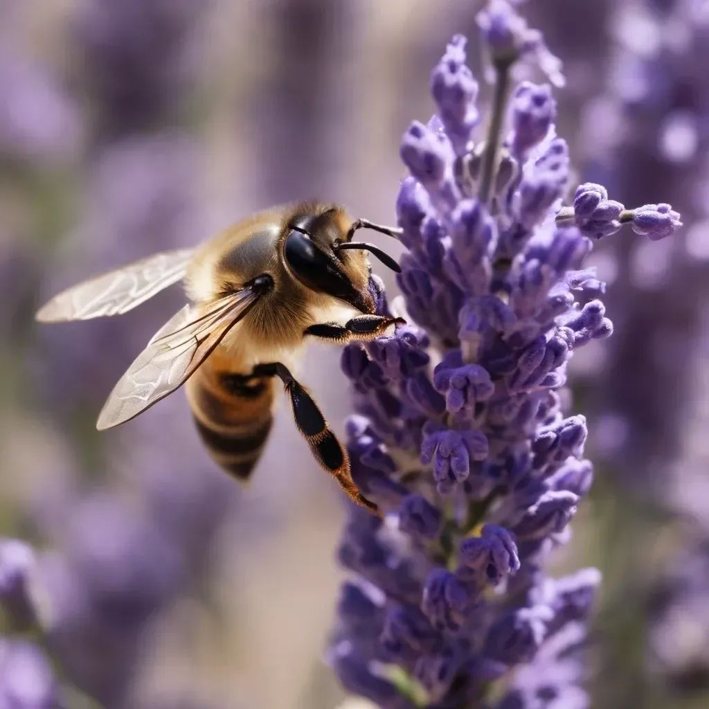
pip install torch torchvision --index-url https://download.pytorch.org/whl/cu118pip install transformers accelerate diffusers

The tests included generating 4 images and comparing different optimization techniques, some of which I believe you may not have seen before. These images of different subjects were generated using the stabilityai/stable-diffusion-xl-base-1.0 model, using only one positive prompt and a fixed seed. The remaining parameters will remain at their default values: no negative prompts, 1024×1024 size, CFG value of 5, and 50 steps (sampling steps).

Prompt and Seed

queue = []# Photorealistic portrait (Portrait)queue.extend([{  'prompt': '3/4 shot, candid photograph of a beautiful 30 year old redhead woman with messy dark hair, peacefully sleeping in her bed, night, dark, light from window, dark shadows, masterpiece, uhd, moody',  'seed': 877866765,}])# Creative interior image (Interior)queue.extend([{  'prompt': 'futuristic living room with big windows, brown sofas, coffee table, plants, cyberpunk city, concept art, earthy colors',  'seed': 5567822456,}])# Macro photography (Macro)queue.extend([{  'prompt': 'macro shot of a bee collecting nectar from lavender flowers',  'seed': 2257899453,}])# Rendered 3D image (3D)queue.extend([{  'prompt': '3d rendered isometric fiji island beach, 3d tile, polygon, cartoony, mobile game',  'seed': 987867834,}])

Here are the images generated by default:

Here are the results of the comparison tests:

• Perceived quality of images (I hope I am a good judge).

• Time taken to generate each image, as well as total compilation time (if any).

• Maximum memory used.

Each test was run 5 times and compared using averages.

The time measurements were structured as follows:

from time import perf_counter# Import libraries# import ...# Define prompts# queue = []# queue.extend ...for i, generation in enumerate(queue, start=1):  # We start the counter  image_start = perf_counter()# Generate and save image  # ...# We stop the counter and save the result  generation['total_time'] = perf_counter() - image_start# Print the generation time of each imageimages_totals = ', '.join(map(lambda generation: str(round(generation['total_time'], 1)), queue))print('Image time:', images_totals)# Print the average timeimages_average = round(sum(generation['total_time'] for generation in queue) / len(queue), 1)print('Average image time:', images_average)

To find out the maximum memory used, the following statement was included at the end of the file:

max_memory = round(torch.cuda.max_memory_allocated(device='cuda') / 1000000000, 2)print('Max. memory used:', max_memory, 'GB')

Each test included only the minimum required code. While each test has its own structure, the code is generally as follows.

# Load the model on the graphics cardpipe = AutoPipelineForText2Image.from_pretrained(  'stabilityai/stable-diffusion-xl-base-1.0',  use_safetensors=True,  torch_dtype=torch.float16,  variant='fp16',).to('cuda')# Create a generatorgenerator = torch.Generator(device='cuda')# Start a loop to process prompts one by onefor i, generation in enumerate(queue, start=1):  # Assign the seed to the generator  generator.manual_seed(generation['seed'])  # Create the image  image = pipe(    prompt=generation['prompt'],    generator=generator,  ).images[0]  # Save the image  image.save(f'image_{i}.png')

To make the tests more realistic and reduce time consumption, all tests will use FP16 optimization.

Many of the tests used the pipeline in the diffusers library to abstract complexity and make the code clearer and more concise. When testing requires, the level of abstraction will be lowered, but ultimately we will always use the methods provided by the library. Additionally, the model is always loaded in safetensors format, using the use_safetensors=True property.

The image sizes displayed in the article are a maximum of 512×512 for browsing, but you can open the images in a new tab/window to view their original sizes.

You can find all individual test files in the article repository on GitHub (github.com/felixsanz/felixsanz_dev).

Let’s get started!

2

Basic Optimization

CUDA and PyTorch Versions

I conducted this test to see if there were differences between using CUDA 11.8 or CUDA 12.1, as well as any potential differences between different versions of PyTorch (always above 2.0).

Test results:

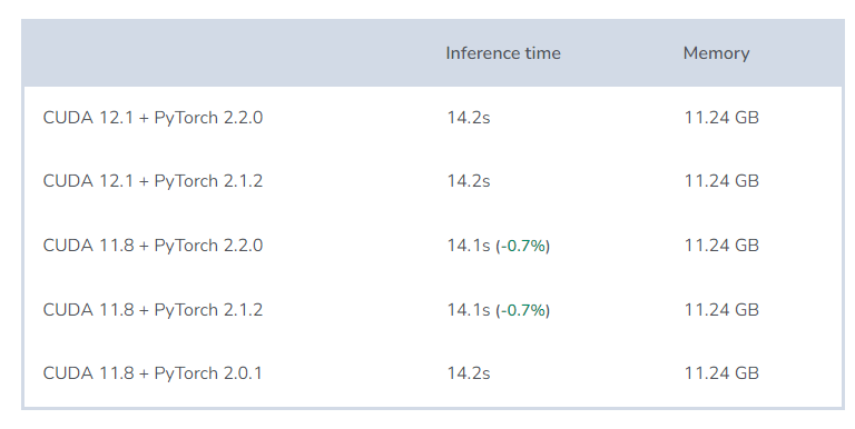
Conclusion:

Disappointingly, their performance was not different. The differences were so small that perhaps if I conducted more tests, this difference would disappear.

When to use: Regarding which version to use, I still have a theory: the CUDA version 11.8 has been released longer, and theoretically, the performance of the libraries and applications in that version should outperform the newer version. On the other hand, for PyTorch, the newer the version, the more features it should provide, and the fewer bugs it should contain. Therefore, even if it is just a psychological effect, I would stick with CUDA 11.8 + PyTorch 2.2.0.

Attention Mechanism

In the past, the attention mechanism had to be optimized by installing libraries such as xFormers or FlashAttention.

If you are curious why this article does not mention the above optimizations, it is because it is no longer necessary. Since the release of PyTorch 2.0, the optimizations of the above algorithms have been integrated into the library through various implementations (such as the two mentioned above). PyTorch will implement appropriately based on the input and the hardware being used.

FP16

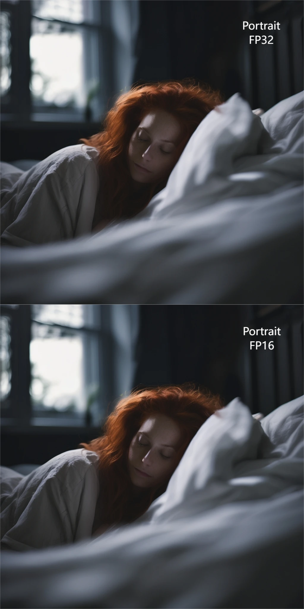
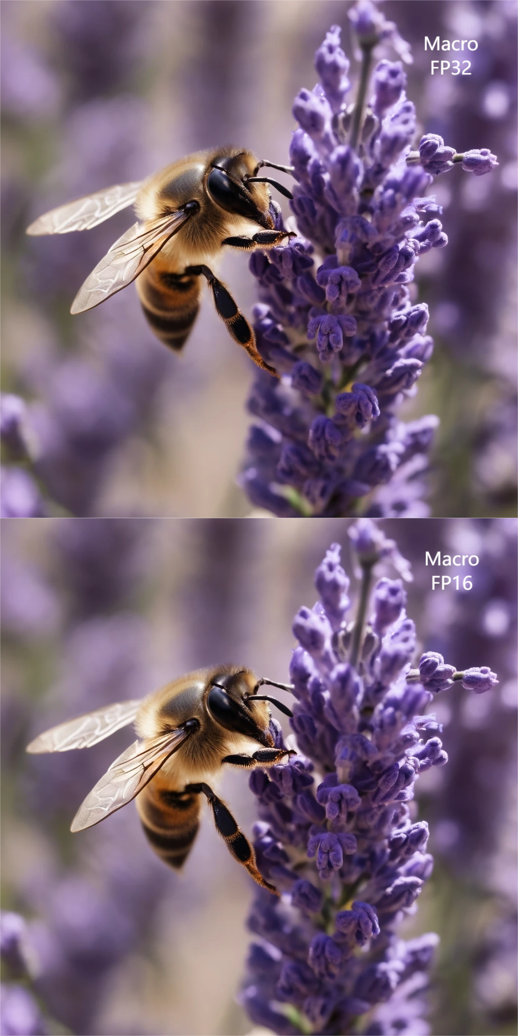
By default, Stable Diffusion XL uses 32 bit floating point format (FP32) to represent the numbers it processes and performs calculations.

An obvious question: can precision be reduced? The answer is yes. By using the parameter torch_dtype=torch.float16, the model will be loaded into memory in half precision floating point format (FP16). To avoid constantly making this conversion, we can directly download the model variant distributed in FP16 format. Just include the variant=’fp16′ parameter.

pipe = AutoPipelineForText2Image.from_pretrained(  'stabilityai/stable-diffusion-xl-base-1.0',  use_safetensors=True,  torch_dtype=torch.float16,  variant='fp16',).to('cuda')generator = torch.Generator(device='cuda')for i, generation in enumerate(queue, start=1):  generator.manual_seed(generation['seed'])  image = pipe(    prompt=generation['prompt'],    generator=generator,  ).images[0]  image.save(f'image_{i}.png')

Test results:

＜Swipe left/right to see more images＞

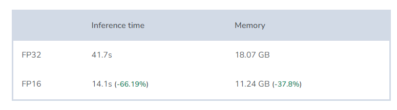
Conclusion:

By using half-precision numbers, memory usage is significantly reduced, and computation speed is greatly improved.

The only “drawback” is the slight reduction in image quality, but in reality, it is almost impossible to see any difference because FP16 is sufficient.

Furthermore, thanks to the variant=’fp16′ parameter, we save disk space, as the variant occupies only half the space of the original (5GB instead of 10GB).

When to use: Always available.

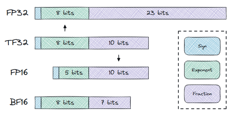
TF32

TensorFloat-32 is a format between FP32 and FP16, allowing certain NVIDIA graphics cards (like A100 or H100) to use tensor cores for calculations. It uses the same bits as FP32 for the exponent, and the same bits as FP16 for the fraction.

Although this format cannot be used for calculations on our test platform (RTX 3090), surprisingly, some very peculiar things happen.

There are two properties to activate this numeric format: torch.backends.cudnn.allow_tf32 (which is enabled by default) and torch.backends.cuda.matmul.allow_tf32 (which should be manually activated). The first property enables TF32 in convolution operations executed by cuDNN, while the second property enables TF32 in matrix multiplication operations.

The torch.backends.cudnn.allow_tf32 property is enabled by default, regardless of what your graphics card is, which is a bit strange. If we disable this property and set it to False, let’s see what happens.

torch.backends.cudnn.allow_tf32 = False# it's already disabled by default# torch.backends.cuda.matmul.allow_tf32 = Falsepipe = AutoPipelineForText2Image.from_pretrained(  'stabilityai/stable-diffusion-xl-base-1.0',  use_safetensors=True,  torch_dtype=torch.float16,  variant='fp16',).to('cuda')generator = torch.Generator(device='cuda')for i, generation in enumerate(queue, start=1):  generator.manual_seed(generation['seed'])  image = pipe(    prompt=generation['prompt'],    generator=generator,  ).images[0]  image.save(f'image_{i}.png')

Additionally, out of curiosity, I also tested with the NVIDIA A100 graphics card that has TF32 enabled.

# it's already activated by default# torch.backends.cudnn.allow_tf32 = Truetorch.backends.cuda.matmul.allow_tf32 = Truepipe = AutoPipelineForText2Image.from_pretrained(  'stabilityai/stable-diffusion-xl-base-1.0',  use_safetensors=True,).to('cuda')generator = torch.Generator(device='cuda')for i, generation in enumerate(queue, start=1):  generator.manual_seed(generation['seed'])  image = pipe(    prompt=generation['prompt'],    generator=generator,  ).images[0]  image.save(f'image_{i}.png')

Trade-off: To use TF32, FP16 format must be disabled, so we cannot use torch_dtype=torch.float16 or variant=’fp16′.

Test results:

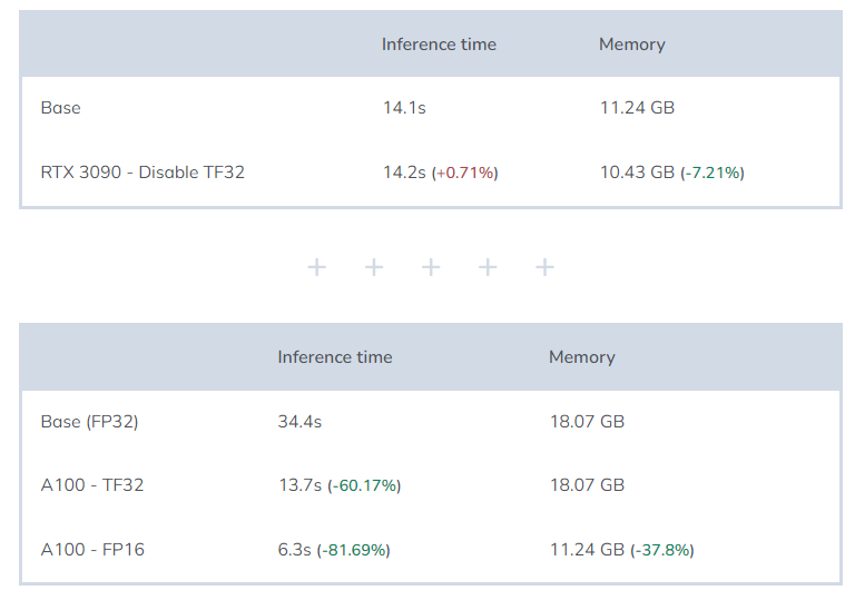
Conclusion::

When using RTX 3090, if the torch.backends.cudnn.allow_tf32 property is disabled, memory consumption decreases by 7%. Why? I don’t know, but in principle, I think this might be a bug because it makes no sense to enable TF32 on a graphics card that does not support TF32.

When using the A100 graphics card, using FP16 can significantly reduce inference time and memory consumption. Just like on the RTX 3090, disabling the torch.backends.cudnn.allow_tf32 property can further reduce memory consumption. As for using TF32, it lies between FP32 and FP16, and it cannot surpass FP16.

When to use: For graphics cards that do not support TF32, it is obviously wise to disable the default enabled property. When using A100, if FP16 can be used, TF32 is not worth using.

3

Pipeline Optimization

The following optimization methods improve the pipeline to enhance performance in certain aspects.

The first three optimizations improve when different components of Stable Diffusion are loaded into memory so that they don’t load simultaneously. These techniques achieve the goal of reducing memory usage.

Use these optimizations when they are needed due to graphics card and memory limitations. If you receive a RuntimeError: CUDA out of memory error on Linux, this section is what you need. On Windows, virtual memory (shared GPU memory) is present by default, and although it is difficult to encounter this error, inference time will increase exponentially, so this section is also what you need to focus on.

As for the last three optimization methods in this section, they optimize the pipeline’s library in different ways to minimize inference time as much as possible.

Model CPU Offload

The Model CPU Offload optimization method comes from the accelerate library. When executing the pipeline, all models are loaded into memory. With this optimization, we allow the pipeline to move the model into memory only when needed each time.

model_cpu_offload_seq = "text_encoder->text_encoder_2->image_encoder->unet->vae"

ImplementingModel CPU Offload is very simple:

pipe = AutoPipelineForText2Image.from_pretrained(  'stabilityai/stable-diffusion-xl-base-1.0',  use_safetensors=True,  torch_dtype=torch.float16,  variant='fp16',).to('cuda')pipe.enable_model_cpu_offload()generator = torch.Generator(device='cuda')for i, generation in enumerate(queue, start=1):  generator.manual_seed(generation['seed'])  image = pipe(    prompt=generation['prompt'],    generator=generator,  ).images[0]  image.save(f'image_{i}.png')

Important Reminder: Unlike other optimizations, we should not use to(‘cuda’) to move the pipeline onto the graphics card. This optimization will be handled automatically when necessary. (Thanks to Terrence Goh for the reminder)

pipe = AutoPipelineForText2Image.from_pretrained(  # ...).to('cuda')

Test results:

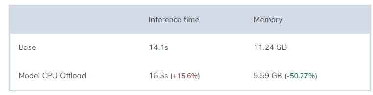
Conclusion:

Using this technique will depend on the graphics card we have: If the graphics card has 6-8GB of memory, this optimization will help, as memory usage is reduced by half.

As for inference time, it will not be significantly affected to become a problem.

When to use: Use when memory consumption needs to be reduced. Since the component that consumes the most memory is the noise predictor (U-Net), we cannot further reduce memory consumption by applying optimizations to the VAE.

Sequential CPU Offload

This optimization is similar to Model CPU Offload, but is more aggressive. It does not move the entire component into memory, but rather moves each submodule of the component into memory. For example, this optimization does not move the entire U-Net model into memory but moves specific parts in and out of memory as needed. This means that if the noise predictor needs to clean a tensor in 50 steps, the submodules must move in and out of memory 50 times.

Just add one line of code:

pipe = AutoPipelineForText2Image.from_pretrained(  'stabilityai/stable-diffusion-xl-base-1.0',  use_safetensors=True,  torch_dtype=torch.float16,  variant='fp16',)pipe.enable_sequential_cpu_offload()generator = torch.Generator(device='cuda')for i, generation in enumerate(queue, start=1):  generator.manual_seed(generation['seed'])  image = pipe(    prompt=generation['prompt'],    generator=generator,  ).images[0]  image.save(f'image_{i}.png')

Important Note: Remember not to use to(‘cuda’) in the pipeline when using Model CPU Offload.

Test results:

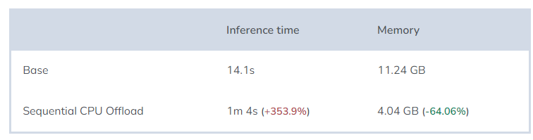
Conclusion:

This optimization will test our patience. To minimize memory usage as much as possible, inference time will increase significantly.

When to use: If you need to keep memory under 4GB, then using this optimization with VAE FP16 fix or Tiny VAE is your only option, but if you don’t need to do so, that’s even better.

Batching

This technique was learned from the articles “How to implement Stable Diffusion” (https://www.felixsanz.dev/articles/how-to-implement-stable-diffusion) and “PixArt-α with less than 8GB VRAM” (https://www.felixsanz.dev/articles/pixart-a-with-less-than-8gb-vram), where I learned about this technique. Through these articles, you will find some code information that I will use but not explain anymore.

This relates to executing components in batching. The idea behind it is similar to the “Model CPU Offload” technique, but the issue is that the official pipeline implementation does not optimize memory usage to the fullest. When you start the pipeline, you cannot just get the text encoder.

That is to say, we should be able to do this:

pipe = AutoPipelineForText2Image.from_pretrained(  'stabilityai/stable-diffusion-xl-base-1.0',  use_safetensors=True,  torch_dtype=torch.float16,  variant='fp16',  unet=None,  vae=None,).to('cuda')

But in reality, this cannot be done. When you start the pipeline, it needs to access U-Net model configurations (self.unet.config.*) and VAE configurations (self.vae.config.*).

Therefore (and without creating a branch), we will manually use the text encoder without relying on the pipeline.

The first step is to copy the encode_prompt function from the pipeline and adjust/simplify it.

This function is responsible for tokenizing the prompt and processing it to obtain the converted embedding tensor. You can find an explanation of this process in “How to implement Stable Diffusion”.

def encode_prompt(prompts, tokenizers, text_encoders):  embeddings_list = []  for prompt, tokenizer, text_encoder in zip(prompts, tokenizers, text_encoders):    cond_input = tokenizer(      prompt,      max_length=tokenizer.model_max_length,      padding='max_length',      truncation=True,      return_tensors='pt',    )    prompt_embeds = text_encoder(cond_input.input_ids.to('cuda'), output_hidden_states=True)    pooled_prompt_embeds = prompt_embeds[0]    embeddings_list.append(prompt_embeds.hidden_states[-2])  prompt_embeds = torch.concat(embeddings_list, dim=-1)  negative_prompt_embeds = torch.zeros_like(prompt_embeds)  negative_pooled_prompt_embeds = torch.zeros_like(pooled_prompt_embeds)  bs_embed, seq_len, _ = prompt_embeds.shape  prompt_embeds = prompt_embeds.repeat(1, 1, 1)  prompt_embeds = prompt_embeds.view(bs_embed * 1, seq_len, -1)  seq_len = negative_prompt_embeds.shape[1]  negative_prompt_embeds = negative_prompt_embeds.repeat(1, 1, 1)  negative_prompt_embeds = negative_prompt_embeds.view(1 * 1, seq_len, -1)  pooled_prompt_embeds = pooled_prompt_embeds.repeat(1, 1).view(bs_embed * 1, -1)  negative_pooled_prompt_embeds = negative_pooled_prompt_embeds.repeat(1, 1).view(bs_embed * 1, -1)  return prompt_embeds, negative_prompt_embeds, pooled_prompt_embeds, negative_pooled_prompt_embeds

Next, we instantiate all necessary components and models. We also need a garbage collector (gc).

import gcfrom transformers import CLIPTokenizer, CLIPTextModel, CLIPTextModelWithProjection# ...tokenizer = CLIPTokenizer.from_pretrained(  'stabilityai/stable-diffusion-xl-base-1.0',  subfolder='tokenizer',)text_encoder = CLIPTextModel.from_pretrained(  'stabilityai/stable-diffusion-xl-base-1.0',  subfolder='text_encoder',  use_safetensors=True,  torch_dtype=torch.float16,  variant='fp16',).to('cuda')tokenizer_2 = CLIPTokenizer.from_pretrained(  'stabilityai/stable-diffusion-xl-base-1.0',  subfolder='tokenizer_2',)text_encoder_2 = CLIPTextModelWithProjection.from_pretrained(  'stabilityai/stable-diffusion-xl-base-1.0',  subfolder='text_encoder_2',  use_safetensors=True,  torch_dtype=torch.float16,  variant='fp16',).to('cuda')

Now we need to combine these two parts. We call the encode_prompt function and pass the same prompt to the first text encoder and the second text encoder, providing components for use.

with torch.no_grad():  for generation in queue:    generation['embeddings'] = encode_prompt(      [generation['prompt'], generation['prompt']],      [tokenizer, tokenizer_2],      [text_encoder, text_encoder_2],    )

The resulting tensor is stored in a variable for later use.

Since we have processed all prompts, we can delete these components from memory:

del tokenizer, text_encoder, tokenizer_2, text_encoder_2gc.collect()torch.cuda.empty_cache()

Now, let’s create a pipeline that can only access U-Net and VAE without needing to instantiate the text encoder to save memory.

pipe = AutoPipelineForText2Image.from_pretrained(  'stabilityai/stable-diffusion-xl-base-1.0',  use_safetensors=True,  torch_dtype=torch.float16,  variant='fp16',  tokenizer=None,  text_encoder=None,  tokenizer_2=None,  text_encoder_2=None,).to('cuda')

Preheating: Since each part is separate, the preheating for this test is a bit complicated. Nevertheless, we will use the following code to preheat the U-Net model:

for generation in queue:  pipe(    prompt_embeds=generation['embeddings'][0],    negative_prompt_embeds =generation['embeddings'][1],    pooled_prompt_embeds=generation['embeddings'][2],    negative_pooled_prompt_embeds=generation['embeddings'][3],    output_type='latent',  )

We use the pipeline to process the embedding tensors saved in the previous step. Remember that in this section, the pipeline creates a tensor filled with noise and cleans it in 50 steps (while guided by our embedding vectors).

generator = torch.Generator(device='cuda')for i, generation in enumerate(queue, start=1):  generator.manual_seed(generation['seed'])  generation['latents'] = pipe(    prompt_embeds=generation['embeddings'][0],    negative_prompt_embeds =generation['embeddings'][1],    pooled_prompt_embeds=generation['embeddings'][2],    negative_pooled_prompt_embeds=generation['embeddings'][3],    generator=generator,    output_type='latent',  ).images # We do not access images[0], but the entire tensor

As you can see, we instruct the pipeline to return the tensor in latent space (output_type=’latent’). If we do not do this, the VAE will be loaded into memory to return the image, which will cause both models to occupy resources simultaneously. So, just like we deleted the text encoder earlier, we delete the U-Net model.

del pipe.unetgc.collect()torch.cuda.empty_cache()

Now we convert the stored denoised tensor into an image:

pipe.upcast_vae()with torch.no_grad():  for i, generation in enumerate(queue, start=1):    generation['latents'] = generation['latents'].to(next(iter(pipe.vae.post_quant_conv.parameters())).dtype)    image = pipe.vae.decode(      generation['latents'] / pipe.vae.config.scaling_factor,      return_dict=False,    )[0]    image = pipe.image_processor.postprocess(image, output_type='pil')[0]    image.save(f'image_{i}.png')

VAE (FP32): In Stable Diffusion XL, we use pipe.upcast_vae() to keep the VAE in FP32 format because it does not work properly in FP16.

This loop is responsible for decoding the tensors in latent space to convert them into image space. Then, using the pipe.image_processor.postprocess method, it is converted into an image and saved.

Test results:

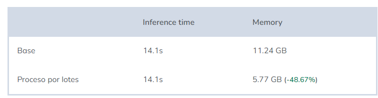
Conclusion:

This is one of the reasons I decided to write this article. Without affecting inference time, we reduced memory usage by half. Now, even a graphics card with only 6GB of memory can generate images.

When to use: Whenever we want to use the refiner model to improve the visual quality of images.

Expert Denoiser Integration

So what about the refiner model? While we have optimized the base model, one of the main advantages of Stable Diffusion XL is that it also has a dedicated model for refining details. This model significantly improves the quality of generated images.

By default, the base model uses 11.24 GB of memory. When using the refiner model simultaneously, the memory requirement increases to 17.38 GB. But remember, since it has the same components (except for the first text encoder), most optimizations can also be applied to this model.

When preheating the refiner model, it becomes a bit complex as it requires preheating two different models. To achieve this, we first obtain results from the base model, and then process them through the refiner model:

for generation in queue:  image = base(generation['prompt'], output_type='latent').images  refiner(generation['prompt'], image=image)

The refiner model can be used in two different ways, which we will discuss separately.

Ensemble of Expert Denoisers

The Ensemble of Expert Denoisers refers to the method of image generation that starts with the base model and ends with the refiner model. Throughout the process, no images are generated, but the base model cleans the tensor within a specified number of steps (a portion of the total steps) and then passes the tensor to the refiner model for completion.

It can be said that they work together to produce results (base model + refiner).

In terms of code, the base model stops its work at 80% of the process using the denoising_end=0.8 parameter and returns the tensor through output_type=’latent’.

The refiner model receives this tensor (ironically, it is not an image) through the image parameter. Then, the refiner model starts to clean this tensor, assuming that it has already completed 80% of the work with the denoising_start=0.8 parameter. We specify the number of steps for the entire processing process (num_inference_steps) so that it calculates the remaining steps that need to be cleaned. That is, if we use 50 steps and change at 80%, the base model will clean the tensor for the first 40 steps, and the refiner model will refine the remaining 10 steps to perfect the remaining details.

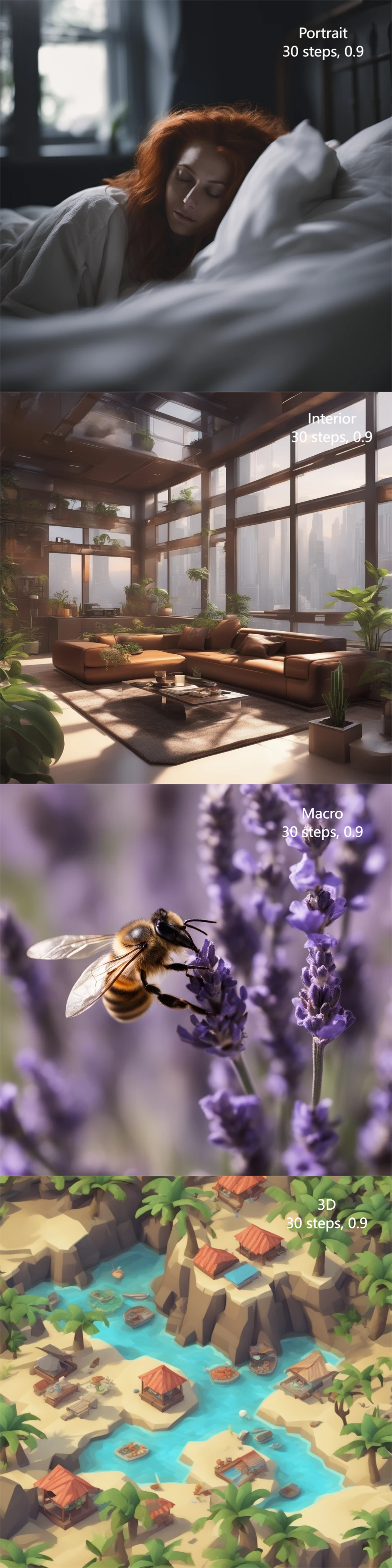
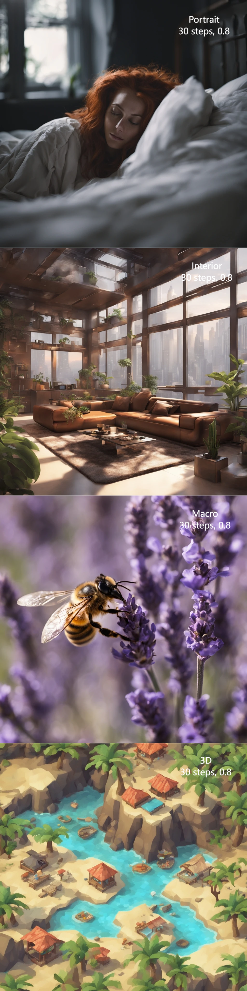
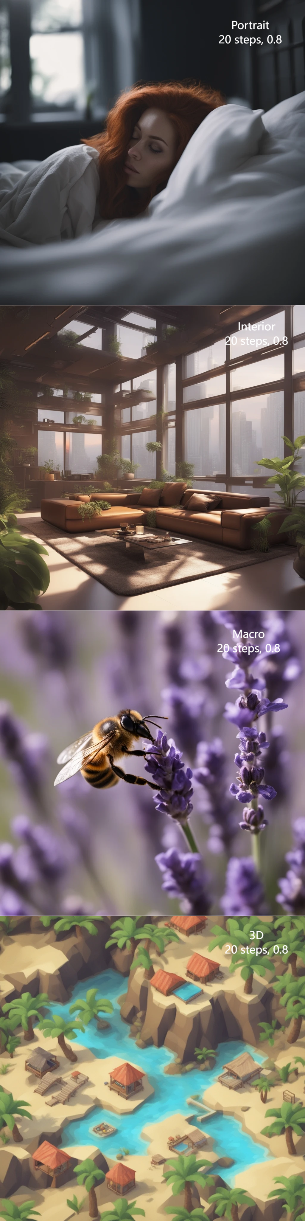
from diffusers import AutoPipelineForText2Image, AutoPipelineForImage2Image# ...base = AutoPipelineForText2Image.from_pretrained(  'stabilityai/stable-diffusion-xl-base-1.0',  use_safetensors=True,  torch_dtype=torch.float16,  variant='fp16',).to('cuda')refiner = AutoPipelineForImage2Image.from_pretrained(  'stabilityai/stable-diffusion-xl-refiner-1.0',  use_safetensors=True,  torch_dtype=torch.float16,  variant='fp16',).to('cuda')generator = torch.Generator(device='cuda')for i, generation in enumerate(queue, start=1):  generator.manual_seed(generation['seed'])  image = base(    prompt=generation['prompt'],    generator=generator,    num_inference_steps=50,    denoising_end=0.8,    output_type='latent',  ).images # Remember that here we do not access images[0], but the entire tensor  image = refiner(    prompt=generation['prompt'],    generator=generator,    num_inference_steps=50,    denoising_start=0.8,    image=image,  ).images[0]  image.save(f'image_{i}.png')

We will generate images at 50, 40, 30, and 20 steps in the base model and then add an extra 20 steps and a combination of 10 steps through the refiner model.

As a reference, we will also include the base image from all comparisons, which is the result processed by the base model, using only 50 steps.

Test results:

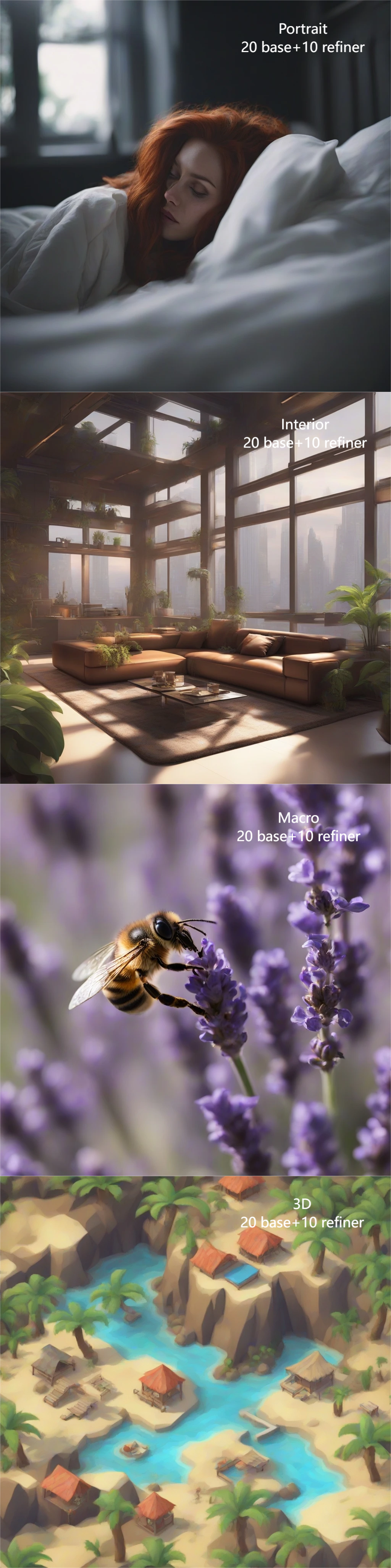
Conclusion:

There is no doubt that using the refiner model will greatly improve the results.

So when should we use the refiner model to process images? Clearly, the results obtained at 0.9 are better than those at 0.8, because the refiner model is designed to optimize final details and should not be used to alter the structure of the image.

I believe that regardless of the number of steps, the refiner model seems to provide very high visual quality results. The only thing that will change is the structure of the image, but even with only 30 steps, the visual quality is high.

At the same time, we must also consider that when the number of steps is reduced to below 40, the required time will decrease significantly.

When to use: Whenever we want to use the refiner model to improve the visual quality of images. As for parameters, we can use 30 or 40 steps as long as we do not pursue the best quality. Of course, we should always switch to the refiner model at 0.9.

Image-to-Image

In Stable Diffusion XL, the classic image-to-image (img2img) method is not new. This method generates a complete image using the base model and then passes the generated image along with the original prompt to the refiner model, which uses these conditions to generate a new image.

In other words, in the img2img method, these two models work independently (base model -> refiner model).

Since the two processes are independent, it is relatively easy to apply the optimization methods in this article. Nevertheless, the code does not differ much, it simply generates an image and uses it as a parameter for the refiner model.

from diffusers import AutoPipelineForText2Image, AutoPipelineForImage2Image# ...base = AutoPipelineForText2Image.from_pretrained(  'stabilityai/stable-diffusion-xl-base-1.0',  use_safetensors=True,  torch_dtype=torch.float16,  variant='fp16',).to('cuda')refiner = AutoPipelineForImage2Image.from_pretrained(  'stabilityai/stable-diffusion-xl-refiner-1.0',  use_safetensors=True,  torch_dtype=torch.float16,  variant='fp16',).to('cuda')generator = torch.Generator(device='cuda')for i, generation in enumerate(queue, start=1):  generator.manual_seed(generation['seed'])  image = base(    prompt=generation['prompt'],    generator=generator,    num_inference_steps=50,  ).images[0]  image = refiner(    prompt=generation['prompt'],    generator=generator,    num_inference_steps=10,    image=image,  ).images[0]  image.save(f'image_{i}.png')

We will generate images at 50, 40, 30, and 20 steps in the base model and then add an extra 20 steps and a combination of 10 steps through the refiner model.

As a reference, we will also include the base image from all comparisons, which is the result processed by the base model, using only 50 steps.

Test results:

Conclusion:

In the image-to-image (img2img) mode, the performance of the refiner model is not satisfactory.

When we use a sufficient number of steps in the base model, it seems that the refiner model is forced to add details to parts that do not need it. In other words, this is adding unnecessary details.

On the other hand, if we use fewer steps in the base model, the results are slightly better. This is because with such a small number of steps, the base model is unable to add subtle details, leaving more room for the refiner model to work.

At the same time, we must also consider that reducing the number of steps will reduce time. If we use too many steps, we will suffer a significant loss.

When to use: First, remember that the purpose of using the refiner model is to maximize visual quality. In this case, we can increase the number of steps, so the “Ensemble of Expert Denoisers” method is the best choice. I believe that using a small number of steps will not yield better visual quality and will not improve generation speed, and compared to other methods, it does not have an advantage. Therefore, using the refiner model in image-to-image mode has its advantages, but they are not prominent.

6

Conclusion

When I started writing this article, I did not expect to delve into it to this extent. I can understand readers who jump straight to the conclusion section, and I also admire those who read all the optimization content. I hope that after reading this article, readers will gain something.

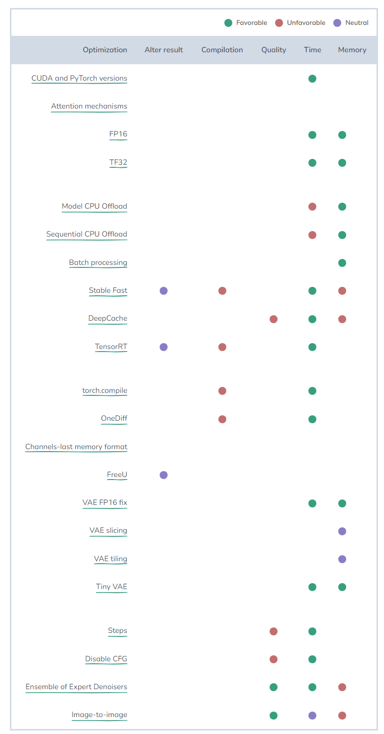
Depending on the goals and available hardware, we need to apply different optimization methods. Let’s summarize all the optimizations and the improvements (or losses) they introduce in tabular form.

Theoretically, a “neutral” optimization method is a beneficial change in this category, but its interpretability may be controversial or only applicable to certain specific use cases.

Fastest Speed

Using the base model combined with OneDiff + Tiny VAE + disabling CFG at 75% + 30 steps, can achieve the shortest generation time with almost no loss in quality, resulting in the fastest speed.

With an RTX 3090 graphics card, images can be generated in just 4.0 seconds, with a memory consumption of 6.91 GB, allowing it to run even on graphics cards with 8 GB of memory.

We can also add DeepCache to speed up the process further, but the problem is that it is incompatible with the disabling CFG optimization; once it is disabled, the final speed will increase.

Using the same configuration, the A100 graphics card can generate images in 2.7 seconds. On the brand new H100, the inference time is only 2.0 seconds.

Memory Usage Under 4GB

When using Sequential CPU Offload, the bottleneck is the VAE. Therefore, combining this optimization with VAE FP16 fix or Tiny VAE will require 2.56 GB and 0.68 GB of memory usage respectively. While the memory usage is ridiculously low, the inference time will make you feel the need to switch to a new graphics card with more memory.

Memory Usage Under 6GB

Once breaking the 6 GB memory limit, new optimization options can be opened.

As previously seen, using OneDiff + Tiny VAE reduces memory usage to 6.91 GB and achieves the lowest possible inference time. Therefore, if your graphics card has at least 8 GB of memory, this may be your best choice.

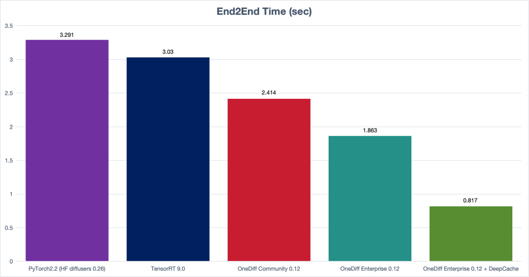
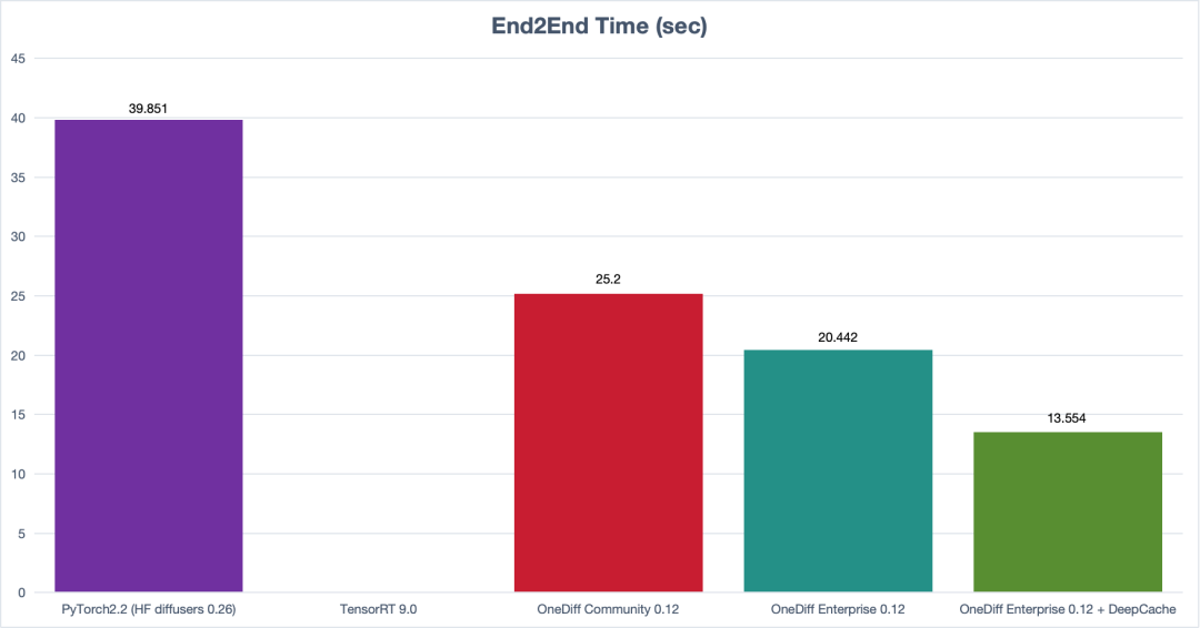
【OneDiff v0.12.1 Official Release (Stable Acceleration for Production Environment SD&SVD)】 This update includes the following highlights, welcome to experience the new version: github.com/siliconflow/onediff

* Update SDXL and SVD’s SOTA performance

* Fully supports dynamic resolution operation for SD and SVD

* Compiling/Saving/Loading HF Diffusers’ pipeline

* Fast LoRA loading and switching for HF Diffusers

* Accelerated InstantID (1.8x faster)

* Accelerated SDXL Lightning

(SDXL E2E Time)

(SVD E2E Time)

More details: https://medium.com/@SiliconFlowAI/

• 800+ pages of free “large model” e-book

• Extreme speed of LLM inference

• The father of reinforcement learning: another possibility towards AGI

• Long time no see! OneFlow 1.0 new version is online

• LLM inference introductory guide②: In-depth analysis of KV caching

• In just 50 seconds, AI turns your call ringtone into a short video

• OneDiff x