Try These 4 Advanced Optimization Techniques in Deep Learning If Your PyTorch Optimizer Isn't Performing Well

Source: DeepHub IMBA

This article is approximately 3700 words long, recommended reading time is over 10 minutes.
This article will introduce four advanced optimization techniques that may outperform traditional methods in certain tasks, especially when faced with complex optimization problems.

In the field of deep learning, the choice of optimizer is crucial for model performance. While standard optimizers in PyTorch such as SGD, Adam, and AdamW are widely used, they are not always the best choice in every scenario. This article will introduce four advanced optimization techniques that may outperform traditional methods, particularly when facing complex optimization problems.

We will explore the following algorithms:

Sequential Least Squares Programming (SLSQP)
Particle Swarm Optimization (PSO)
Covariance Matrix Adaptation Evolution Strategy (CMA-ES)
Simulated Annealing (SA)

The main advantages of these methods include:

Gradient-free optimization: Suitable for non-differentiable operations such as sampling, rounding, and combinatorial optimization.
Only requires forward propagation: Generally faster and more memory efficient than traditional methods.
Global optimization capability: Helps avoid local optima.

It is important to note that these methods are best suited for optimizing a smaller number of parameters (typically less than 100-1000). They are particularly useful for optimizing key parameters, specific parameters per layer, or hyperparameters.

Experimental Setup

Before starting the experiments, we need to set up the environment and define some auxiliary functions. Below are the necessary imports and function definitions:

 from functools import partial
from collections import defaultdict
import torch
import torch.nn as nn
import torch.optim as optim
import torch.nn.functional as F
import numpy as np
import scipy.optimize as opt
import matplotlib.pyplot as plt

# Set random seed for reproducibility
torch.manual_seed(42)
np.random.seed(42)

# Auxiliary function: convert weights between PyTorch model and NumPy vector
def set_model_weights_from_vector(model, numpy_vector):
    weight_vector = torch.tensor(numpy_vector, dtype=torch.float64)
    model[0].weight.data = weight_vector[0:4].reshape(2, 2)
    model[2].weight.data = weight_vector[4:8].reshape(2, 2)
    model[2].bias.data = weight_vector[8:10]
    return model

def get_vector_from_model_weights(model):
    return torch.cat([
        model[0].weight.data.view(-1),
        model[2].weight.data.view(-1),
        model[2].bias.data
    ]).detach().numpy()

# Function to track and update loss

def update_tracker(loss_tracker, optimizer_name, loss_val):
    loss_tracker[optimizer_name].append(loss_val)
    if len(loss_tracker[optimizer_name]) > 1:
        min_loss = min(loss_tracker[optimizer_name][-2], loss_val)
        loss_tracker[optimizer_name][-1] = min_loss
    return loss_tracker

These functions will be used to convert model weights between different optimization algorithms and track the loss during the optimization process.

Next, we define the objective function and the PyTorch optimization loop:

 def objective(x, model, input, target, loss_tracker, optimizer_name):
    model = set_model_weights_from_vector(model, x)
    loss_val = F.mse_loss(model(input), target).item()
    loss_tracker = update_tracker(loss_tracker, optimizer_name, loss_val)
    return loss_val

def pytorch_optimize(x, model, input, target, maxiter, loss_tracker, optimizer_name="Adam"):
    set_model_weights_from_vector(model, x)
    optimizer = optim.Adam(model.parameters(), lr=1.)

    # Training loop
    for iteration in range(maxiter):
        loss = F.mse_loss(model(input), target)
        optimizer.zero_grad()
        loss.backward()
        optimizer.step()
        loss_tracker = update_tracker(loss_tracker, optimizer_name, loss.item())
    final_x = get_vector_from_model_weights(model)
    return final_x, loss.item()

Finally, we set up the common variables required for the experiment:

 model = nn.Sequential(nn.Linear(2, 2, bias=False), nn.ReLU(), nn.Linear(2, 2, bias=True)).double()
input_tensor = torch.randn(32, 2).double()  # Random input tensor
input_tensor[:, 1] *= 1e3  # Increase sensitivity of one variable
target = input_tensor.clone() # The target is the input itself (identity function)
num_params = 10
maxiter = 100
x0 = 0.1 * np.random.randn(num_params)
loss_tracker = defaultdict(list)

These setups create a simple neural network model for our experiment, defining the input, target, and initial parameters.

In the next section, we will begin implementing and comparing different optimization techniques.

Comparison of Optimization Techniques

1. Adam Optimizer in PyTorch

As a baseline, we first use PyTorch’s Adam optimizer. Adam is an adaptive learning rate optimization algorithm widely used in deep learning.

 optimizer_name = "PyTorch Adam"
result = pytorch_optimize(x0, model, input_tensor, target, maxiter, loss_tracker, optimizer_name)
print(f'Final loss with Adam optimizer: {result[1]}')

After running this code, we get the following result:

 Final loss with Adam optimizer: 91.85612831226527

Considering the initial loss value was around 300,000, this result shows significant improvement after 100 optimization steps.

2. Sequential Least Squares Programming (SLSQP)

Sequential Least Squares Programming (SLSQP) is a powerful optimization algorithm particularly suitable for problems with continuous parameters. It approximates the optimal solution by constructing a quadratic approximation at each step.

 optimizer_name = "slsqp"
args = (model, input_tensor, target, loss_tracker, optimizer_name)
result = opt.minimize(objective, x0, method=optimizer_name, args=args, options={"maxiter": maxiter, "disp": False, "eps": 0.001})
print(f"Final loss with SLSQP optimizer: {result.fun}")

After running the SLSQP algorithm, we obtain the following result:


 Final loss with SLSQP optimizer: 3.097042282788268

The performance of SLSQP significantly outperforms Adam, indicating that in some cases, non-traditional optimization methods may be more effective.

3. Particle Swarm Optimization (PSO)

Particle Swarm Optimization (PSO) is an optimization algorithm inspired by the social behavior of birds and fish. PSO performs particularly well on non-continuous and non-smooth problems.

 from pyswarm import pso
lb = -np.ones(num_params)
ub = np.ones(num_params)
optimizer_name = 'pso'
args = (model, input_tensor, target, loss_tracker, optimizer_name)
result_pso = pso(objective, lb, ub, maxiter=maxiter, args=args)
print(f"Final loss with PSO optimizer: {result_pso[1]}")

The optimization result with PSO is as follows:

 Final loss with PSO optimizer: 1.0195048385714032

The performance of PSO further surpasses SLSQP, highlighting the importance of exploring multiple algorithms in complex optimization problems.

4. Covariance Matrix Adaptation Evolution Strategy (CMA-ES)

Covariance Matrix Adaptation Evolution Strategy (CMA-ES) is a highly sophisticated optimization algorithm, particularly suitable for challenging non-convex optimization problems. It guides the search process by adaptively learning the covariance structure of the problem.

 from cma import CMAEvolutionStrategy
es = CMAEvolutionStrategy(x0, 0.5, {"maxiter": maxiter, "seed": 42})
optimizer_name = 'cma'
args = (model, input_tensor, target, loss_tracker, optimizer_name)
while not es.stop():
    solutions = es.ask()
    object_vals = [objective(x, *args) for x in solutions]
    es.tell(solutions, object_vals)
print(f"Final loss with CMA-ES optimizer: {es.result[1]}")

The optimization result with CMA-ES is as follows:

 (5_w,10)-aCMA-ES (mu_w=3.2,w_1=45%) in dimension 10 (seed=42, Thu Oct 12 22:03:53 2024)
   Final loss with CMA-ES optimizer: 4.084718909553896

Although CMA-ES did not achieve the best performance on this specific problem, it typically excels in handling highly complex multi-modal optimization problems.

5. Simulated Annealing (SA)

Simulated Annealing (SA) is an optimization algorithm inspired by metallurgy, simulating the cooling and annealing process of metals. SA is particularly effective in finding global optimal solutions, capable of avoiding local optima.

 from scipy.optimize import dual_annealing
bounds = [(-1, 1)] * num_params
optimizer_name = 'simulated_annealing'
args = (model, input_tensor, target, loss_tracker, optimizer_name)
result = dual_annealing(objective, bounds, maxiter=maxiter, args=args, initial_temp=1.)
print(f"Final loss with SA optimizer: {result.fun}")

The optimization result with SA is as follows:

 Final loss with SA optimizer: 0.7834294257939689

As we can see, SA performed the best for our problem, highlighting its potential in complex optimization scenarios.

Next, we will visualize the performance of these optimizers and discuss the implications of the results.

Results Visualization and Analysis

To better understand the performance of various optimization algorithms, we will use the matplotlib library to visualize the change in loss during the optimization process.

 plt.figure(figsize=(10, 6))
line_styles = ['-', '--', '-.', ':']
for i, (optimizer_name, losses) in enumerate(loss_tracker.items()):
    plt.plot(np.linspace(0, maxiter, len(losses)), losses,
             label=optimizer_name,
             linestyle=line_styles[i % len(line_styles)],
             linewidth=5,
    )
plt.xlabel("Iteration", fontsize=20)
plt.ylabel("Loss", fontsize=20)
plt.ylim(1e-1, 1e7)
plt.yscale('log')
plt.title("Loss For Different Optimizers", fontsize=20)
plt.grid(True, linestyle='--', alpha=0.6)
plt.legend(loc='upper right', fontsize=20)
plt.tight_layout()
plt.savefig('optimizers.png')
plt.show()

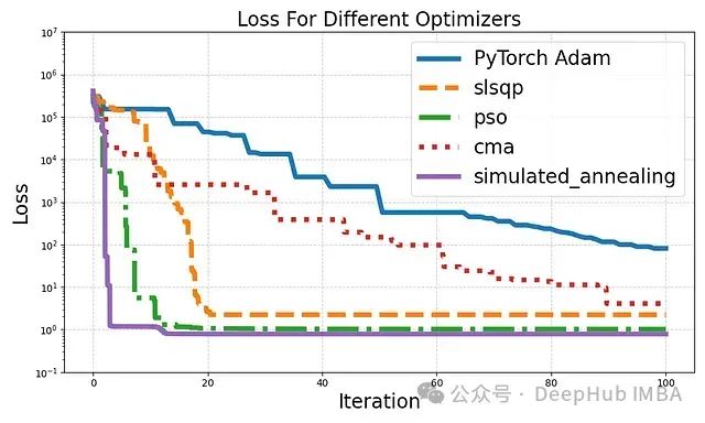
After executing the above code, we obtained the following visualization results:

Results Analysis

Adam Optimizer: As a baseline, Adam performs steadily but has a relatively slow convergence speed. This reflects that traditional gradient descent methods may not be the optimal choice in certain complex problems.
SLSQP: Sequential Least Squares Programming shows rapid initial convergence, indicating its effectiveness in handling problems with continuous parameters.
PSO: Particle Swarm Optimization demonstrates good global search capability, quickly finding better solutions. This highlights its potential in non-convex optimization problems.
CMA-ES: Although it converged slowly in this experiment, the Covariance Matrix Adaptation Evolution Strategy generally excels in handling highly complex and multi-modal problems. Its performance may be more pronounced in more complex optimization scenarios.
Simulated Annealing: In this specific problem, SA performed the best, achieving the lowest loss in just a few iterations. This highlights its advantages in avoiding local optima and quickly finding global optimal solutions.

It is important to note that the definition of “iterations” may vary for each algorithm, so directly comparing iteration counts may not be entirely fair. For example, each iteration of SA may contain multiple evaluations of the objective function.

Conclusion

In specific problems, non-traditional optimization methods may outperform standard gradient descent algorithms (like Adam). However, this does not mean that these methods are superior in all cases. The choice of the most suitable optimization algorithm should be based on the characteristics of the specific problem:

For optimization problems with a smaller number of parameters (100-1000), consider trying the advanced optimization techniques introduced in this article.
When dealing with non-differentiable operations or complex loss landscapes, gradient-free methods (such as PSO, CMA-ES, and SA) may have advantages.
For optimization problems that require complex constraints, SLSQP may be a good choice.
When computational resources are limited, consider using methods that only require forward propagation, such as PSO or SA.
For highly non-convex problems, CMA-ES and SA may be more likely to find global optimal solutions.

Finally, it is recommended to compare and test multiple optimization methods in practical applications to find the algorithm that best fits the specific problem. Also, note that these advanced methods may face computational efficiency challenges on large-scale problems (with more than 1000 parameters).

Future Research Directions

Explore the application of these advanced optimization techniques in more complex deep learning models.
Research how to effectively combine these methods with traditional gradient descent algorithms to develop hybrid optimization strategies.
Develop more efficient parallel implementations to improve the applicability of these algorithms on large-scale problems.
Explore the potential applications of these methods in specific fields (such as reinforcement learning, neural architecture search).

By deeply understanding and flexibly applying these advanced optimization techniques, researchers and engineers can expand the range of solutions when facing complex optimization problems, potentially unlocking new levels of performance and application possibilities.

References

Hansen, N. (2016). The CMA Evolution Strategy: A Tutorial. arXiv preprint arXiv:1604.00772.
Kennedy, J., & Eberhart, R. (1995). Particle swarm optimization. Proceedings of ICNN’95 – International Conference on Neural Networks, 4, 1942-1948.
Nocedal, J., & Wright, S. J. (1999). Numerical Optimization. New York: Springer.
Tsallis, C., & Stariolo, D. A. (1996). Generalized simulated annealing. Physica A: Statistical Mechanics and its Applications, 233(1-2), 395-406.
Kingma, D. P., & Ba, J. (2014). Adam: A Method for Stochastic Optimization. arXiv preprint arXiv:1412.6980.
Ruder, S. (2016). An overview of gradient descent optimization algorithms. arXiv preprint arXiv:1609.04747.

Editor: Huang Jiyan

About Us

Data Hub THU, as a data science public account, backed by the Tsinghua University Big Data Research Center, shares cutting-edge research dynamics in data science and big data technology innovation, continuously disseminates knowledge in data science, strives to build a platform for gathering data talents, and aims to create the strongest group in China’s big data.

Sina Weibo: @Data Hub THU

WeChat Video Account: Data Hub THU

Today’s Headlines: Data Hub THU

Try These 4 Advanced Optimization Techniques in Deep Learning If Your PyTorch Optimizer Isn’t Performing Well