Building DINO Model and PyTorch from Scratch: Self-Supervised Vision Transformer

Click the above“Beginner Learning Vision” to choose to add Star or Pin.

Important content delivered at the first time

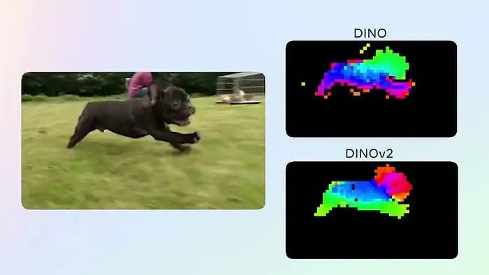
Dog Sprint Output from DINO Model

Unlabeled Self-Distillation (DINO)

The article “Reconstructing Complete Images from Several ‘Patches’ | Building Scalable Learners with Masked Autoencoders” discusses how to build scalable learners, continuing my series on vision transformers, where I explain the most important architectures and their implementation from scratch.

Self-Supervised Learning

Self-supervised learning (SSL) is a type of machine learning where the model learns to understand the data through examples that do not require manual labeling. Instead, it generates its supervisory signals from the data itself. This method is particularly beneficial when labeled data is limited and costly to obtain. In SSL, the learning process involves creating tasks where the input data can be used to predict certain parts of the data itself. Common techniques include:

• Contrastive Learning: The model learns by distinguishing between similar and dissimilar pairs of data.

• Prediction Tasks: The model predicts a part of the input data from other parts, such as predicting the next word in a sentence or predicting the context of a word from its surrounding environment.

DINO Model

The DINO (self-distillation without labels) model is a cutting-edge self-supervised learning method applied to vision transformers (ViTs). It represents a significant advancement in the field of computer vision, enabling models to learn effective image representations without any labeled data. Developed by researchers at Facebook AI Research (FAIR), DINO utilizes a student-teacher framework and innovative training techniques to achieve outstanding performance across various visual tasks.

Student-Teacher Network

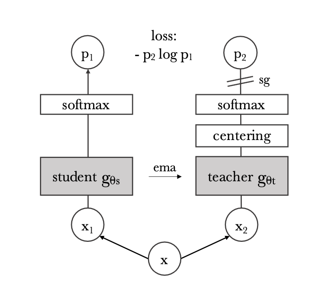
In the DINO model, the student-teacher network is the core mechanism for achieving self-supervised learning without labeled data. This framework involves two networks: the student network and the teacher network. Both networks are vision transformers designed to process images by treating them as sequences of patches, similar to how transformers process sequences of text.

The student network’s task is to learn to generate meaningful representations from the input image. On the other hand, the teacher network provides target representations that the student network aims to match. The teacher network is not a static entity; it evolves over time by gradually integrating the parameters of the student network. This is done through a technique called exponential moving average, where the teacher’s parameters are updated to a weighted average of its current parameters and the student parameters.

The goal is to minimize the difference between the student representations and the teacher representations, which are for the same augmented views of the image. This is typically achieved using a loss function that encourages alignment between the student and teacher outputs while ensuring that representations for different images remain distinct.

By continuously updating the teacher network based on the student network’s learning progress and training the student network to match the teacher’s outputs, DINO effectively leverages the strengths of both networks. The teacher network provides a stable and consistent target for the student, while the student network drives the learning process. This collaborative setup allows the model to learn robust and invariant features from the data without manual labels, enabling effective self-supervised learning.

Augmented Inputs for Student and Teacher

In the DINO model, X1 and X2 (see above) refer to different augmented views of the same original image X. These views serve as inputs for the student and teacher networks, respectively. The goal is for the student network to learn to produce consistent representations under these augmentations. The student and teacher models receive different augmentations based on the following strategies:

• Global Cropping: Create two global crops from the original image. These are larger crops that cover most of the image and typically have a high overlap with the original image, along with other augmentations such as color jittering, Gaussian blur, flipping, etc.

• Local Cropping: In addition to global crops, the teacher network also receives several local crops. These are smaller crops that focus on different parts of the image, capturing more local details.

We will define these augmentations for parameter images that contain a batch of images we want to transform during training.

# These augmentations are defined exactly as proposed in the paper
def global_augment(images):
    global_transform = transforms.Compose([
        transforms.RandomResizedCrop(224, scale=(0.4, 1.0)),  # Larger crops
        transforms.RandomHorizontalFlip(),
        transforms.ColorJitter(0.4, 0.4, 0.4, 0.1),  # Color jittering
        transforms.RandomGrayscale(p=0.2),
        transforms.GaussianBlur(kernel_size=23, sigma=(0.1, 2.0)),
        transforms.ToTensor(),
        transforms.Normalize(mean=[0.485, 0.456, 0.406], std=[0.229, 0.224, 0.225]),
    ])
    return torch.stack([global_transform(img) for img in images])
def multiple_local_augments(images, num_crops=6):
    size = 96  # Smaller crops for local
    local_transform = transforms.Compose([
        transforms.RandomResizedCrop(size, scale=(0.05, 0.4)),  # Smaller, more concentrated crops
        transforms.RandomHorizontalFlip(),
        transforms.ColorJitter(0.4, 0.4, 0.4, 0.1),  # Same level of jittering
        transforms.RandomGrayscale(p=0.2),
        transforms.GaussianBlur(kernel_size=23, sigma=(0.1, 2.0)),
        transforms.ToTensor(),
        transforms.Normalize(mean=[0.485, 0.456, 0.406], std=[0.229, 0.224, 0.225]),
    ])
    # Apply the transformation multiple times to the same image
    return torch.stack([local_transform(img) for img in images])

Distillation Loss:

Here, we want to calculate the loss between the student and teacher outputs using some distance metric. We do this by:

1. Obtaining the centered softmax of the teacher’s predicted outputs and then applying sharpening.

2. Obtaining the student’s softmax predictions and then applying sharpening.

def distillation_loss(student_output, teacher_output, center, tau_s, tau_t):
        """
        Calculates distillation loss with centering and sharpening (function H in pseudocode).
        """
        # Detach teacher output to stop gradients.
        teacher_output = teacher_output.detach()
        # Center and sharpen teacher's outputs
        teacher_probs = F.softmax((teacher_output - center) / tau_t, dim=1)
        # Sharpen student's outputs
        student_probs = F.log_softmax(student_output / tau_s, dim=1)
        # Calculate cross-entropy loss between students' and teacher's probabilities.
        loss = - (teacher_probs * student_probs).sum(dim=1).mean()
        return loss

Centering: Centering the teacher’s outputs ensures that the student model focuses more on the most significant features or distinctions in the teacher output distribution. By centering the distribution, it encourages the student to pay more attention to the salient features crucial for accurate predictions rather than being influenced by variations or biases in the data. This aids in more effective knowledge transfer and can potentially lead to improved performance of the student model.

Sharpening: Sharpening involves amplifying specific features in the data distribution, aiming to highlight the distinctions prominent in the teacher model. This process allows the student model to focus on learning the complex details present in the teacher’s predictions, which is critical for accurately replicating its outputs on the dataset.

Training the DINO Model:

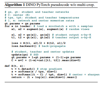
Illustration of DINO pseudocode, taken from the official paper

There are three important steps to highlight:

1. Obtain augmented inputs (x1, x2) for the student and teacher architectures.

2. The distillation loss function we discussed earlier, noting how it computes the distillation loss for the different augmented inputs, i.e., gs({x1, x2}) and gt({x1, x2}).

3. Update (a) student parameters (b) teacher parameters and (c) center. The key here is that we perform exponential moving average updates on the teacher parameters.

• Teacher Parameters: EMA is applied to the parameters of the teacher model. Instead of directly updating the teacher parameters in each training iteration, the EMA maintains a moving average of these parameters over time. This moving average serves as a smoother and more stable representation of the teacher model, which can help guide the training of the student model.

• Center: Additionally, in some implementations of DINO, EMA is also used to update the center. The center represents the mean of the teacher output distribution for normalization purposes. By applying EMA to update the center, it gradually evolves throughout the training process, providing a more stable reference point for normalization.

DINO Model

class DINO(nn.Module):
    def __init__(self, student_arch: Callable, teacher_arch: Callable, device: torch.device):
        """
        Args:
            student_arch (nn.Module): ViT Network for student_arch
            teacher_arch (nn.Module): ViT Network for teacher_arch
            device: torch.device ('cuda' or 'cpu')
        """
        super(DINO, self).__init__()
        self.student = student_arch().to(device)
        self.teacher = teacher_arch().to(device)
        self.teacher.load_state_dict(self.student.state_dict())
        # Initialize center as buffer to avoid backpropagation
        self.register_buffer('center', torch.zeros(1, student_arch().output_dim))
        # Ensure the teacher parameters do not get updated during backprop
        for param in self.teacher.parameters():
            param.requires_grad = False
    @staticmethod
    def distillation_loss(student_output, teacher_output, center, tau_s, tau_t):
        """
        Calculates distillation loss with centering and sharpening (function H in pseudocode).
        """
        # Detach teacher output to stop gradients.
        teacher_output = teacher_output.detach()
        # Center and sharpen teacher's outputs
        teacher_probs = F.softmax((teacher_output - center) / tau_t, dim=1)
        # Sharpen student's outputs
        student_probs = F.log_softmax(student_output / tau_s, dim=1)
        # Calculate cross-entropy loss between student's and teacher's probabilities.
        loss = - (teacher_probs * student_probs).sum(dim=1).mean()
        return loss
    def teacher_update(self, beta: float):
        for teacher_params, student_params in zip(self.teacher.parameters(), self.student.parameters()):
            teacher_params.data.mul_(beta).add_(student_params.data, alpha=(1 - beta))

To update the teacher’s parameters, we use the formula proposed in the paper, i.e., gt.param = gt.param*beta + gs.param*(1 — beta), where beta is the moving average decay, gt and gs are the corresponding teacher and student architectures.

Furthermore, we see that in __init__, the teacher’s parameters are set to “required_grads = False” because we do not want them updated during backpropagation, but rather apply moving average updates.

Additionally, initializing variables as buffers in PyTorch is a common method to keep them outside the gradient graph and not participate in backpropagation.

DINO Model Further Needs the Following Call

device = 'cuda' if torch.cuda.is_available() else 'cpu'
dino = DINO(ViT(), ViT(), device)

Here, we pass the student and teacher architectures, which are just standard vision transformers, i.e., ViT-B/16 or ViT-L/16, as proposed in the first paper.

Final Training

Now the entire implementation can be placed into the training loop, as proposed in the paper.

def train_dino(dino: DINO,
               data_loader: DataLoader,
               optimizer: Optimizer,
               device: torch.device,
               num_epochs,
               tps=0.9,
               tpt= 0.04,
               beta= 0.9,
               m= 0.9,
               ):        
        """
        Args:
            dino: DINO Module
            data_loader (nn.Module): Dataloader for training
            optimizer (nn.optimizer): Optimizer for optimization (SGD etc.)
            defice (torch.device): 'cuda', 'cpu'
            num_epochs: Number of Epochs
            tps (float): tau for sharpening student logits
            tpt: for sharpening teacher logits
            beta (float): moving average decay
             m (float): center moving average decay
        """
            for epoch in range(num_epochs):
            print(f"Epoch: {epoch+1}/{len(num_epochs)}")
            for x in data_loader:
                x1, x2 = global_augment(x), multiple_local_augments(x)  
                student_output1, student_output2 = dino.student(x1.to(device)), dino.student(x2.to(device))
                with torch.no_grad():
                    teacher_output1, teacher_output2 = dino.teacher(x1.to(device)), dino.teacher(x2.to(device))
                # Compute distillation loss
                loss = (dino.distillation_loss(teacher_output1, student_output2, dino.center, tps, tpt) +
                        dino.distillation_loss(teacher_output2, student_output1, dino.center, tps, tpt)) / 2
                # Backpropagation
                optimizer.zero_grad()
                loss.backward()
                optimizer.step()
                # Update the teacher network parameters
                dino.teacher_update(beta)                                
                # Update the center
                with torch.no_grad():
                    dino.center = m * dino.center + (1 - m) * torch.cat([teacher_output1, teacher_output2], dim=0).mean(dim=0)

1. We compute x1 and x2 with different global and local augmentations.

2. Next, we obtain outputs for the student and teacher models based on the methods proposed in the paper, recalling the algorithm flowchart above.

3. Here, we set torch to no_grad() to ensure that the teacher’s parameters are not updated through backpropagation.

4. Finally, we compute the distillation loss again based on the methods proposed in the paper.

5. In the distillation loss, we first center the teacher model’s outputs so that the student model does not easily collapse and does not learn only unimportant features or learn one feature more than another, but focuses on learning the most unique and potential features from the teacher model.

6. Then we sharpen the features so that when calculating the loss, we can now compare two features (student and teacher) that have very different data distributions, meaning that after sharpening, more important features will be emphasized while less important features will not, creating a more unique feature map that makes it easier for the student to learn.

7. We then perform backpropagation and execute optimizer.step() to update the student model and update the teacher network through the previously implemented exponential moving average.

8. As a final step, we set torch to no_grad() again and update the center through moving average. We update the center based on the teacher’s outputs, keeping it consistent with the changes in the output data distribution throughout the training process.

That’s it! This is how to train the DINO model from scratch. So far, in the vision transformer series, we have implemented standard ViT, Swin, CvT, Mae, and DINO (self-supervised). Hope you enjoyed reading this article.

# Create your own CustomDataset and dataloader
dataloader = DataLoader(CustomDataset, batch_size=32, shuffle=True)
optimizer = torch.optim.AdamW(dino.parameters(), lr=1e-4)
train_dino(dino,           DataLoader=dataloader,           Optimizer=optimizer,           device=device,           num_epochs=300,           tps=0.9,           tpt= 0.04,           beta= 0.9,           m= 0.9)

Download 1: OpenCV-Contrib Extension Module Chinese Version Tutorial

Reply "Extension Module Chinese Tutorial" in the "Beginner Learning Vision" public account backend to download the first OpenCV extension module tutorial in Chinese, covering installation of extension modules, SFM algorithms, stereo vision, object tracking, biological vision, super-resolution processing, and more than twenty chapters of content.

Download 2: Python Vision Practical Project 52 Lectures

Reply "Python Vision Practical Project" in the "Beginner Learning Vision" public account backend to download 31 vision practical projects, including image segmentation, mask detection, lane line detection, vehicle counting, eyeliner addition, license plate recognition, character recognition, emotion detection, text content extraction, face recognition, etc., to help quickly learn computer vision.

Download 3: OpenCV Practical Projects 20 Lectures

Reply "OpenCV Practical Projects 20 Lectures" in the "Beginner Learning Vision" public account backend to download 20 practical projects based on OpenCV, achieving advanced learning of OpenCV.

Group Chat

Welcome to join the public account reader group to communicate with peers. Currently, there are WeChat groups for SLAM, 3D vision, sensors, autonomous driving, computational photography, detection, segmentation, recognition, medical imaging, GAN, algorithm competitions, etc. (will be gradually subdivided in the future). Please scan the WeChat ID below to join the group, note: "Nickname + School/Company + Research Direction", for example: "Zhang San + Shanghai Jiao Tong University + Vision SLAM". Please follow the format for notes; otherwise, it will not be approved. After successful addition, you will be invited to the relevant WeChat group based on your research direction. Please do not send advertisements in the group; otherwise, you will be removed from the group. Thank you for your understanding.~