Click on "Xiaobai Learns Vision" above, select "Star" or "Pin"
Heavy content delivered immediately
Editor’s Recommendation
A simple summary is whether it is supervised (supervised) or not, which depends on whether the input data has labels (label). If the input data has labels, it is supervised learning; if there are no labels, it is unsupervised learning.
Reprinted from丨Mathematics China
Machine learning is divided into two main categories based on model type: supervised learning models and unsupervised learning models:
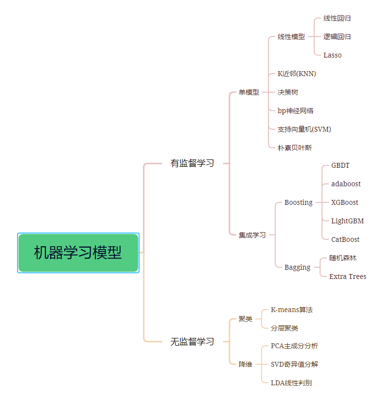
1. Supervised Learning
Supervised learning typically utilizes training data with expert-labeled tags to learn a function mapping from input variable X to output variable Y. Y = f (X), where the training data is usually in the form of (n×x,y), with n representing the size of the training samples, and x and y being the sample values of variables X and Y, respectively.
Supervised learning can be divided into two categories:
-
Classification Problem: Predicting the category (discrete) to which a sample belongs. For example, determining gender, health status, etc.
-
Regression Problem: Predicting the corresponding real number output (continuous) for a sample. For example, predicting the average height of people in a certain area.
In addition, ensemble learning is also a type of supervised learning. It combines predictions from multiple relatively weak machine learning models to predict new samples.
1.1 Single Model
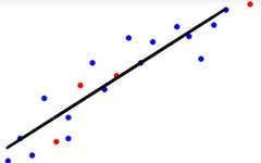
1.11 Linear Regression
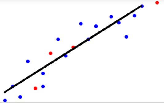
Linear regression refers to a regression model composed entirely of linear variables. In linear regression analysis, there is only one independent variable and one dependent variable, and the relationship between them can be approximated by a straight line, which is called univariate linear regression analysis. If the regression analysis includes two or more independent variables, and the relationship between the dependent and independent variables is linear, it is called multivariate linear regression analysis.
1.12 Logistic Regression

Used to study the relationship between Y as categorical data and X and Y, if Y has two categories like 0 and 1 (for example, 1 means willing and 0 means not willing, 1 means purchase and 0 means no purchase), it is called binary logistic regression; if Y has three or more categories, it is called multi-class logistic regression.
The independent variable does not necessarily have to be categorical; they can also be quantitative variables. If X is categorical data, dummy variable coding is needed for X.
1.13 Lasso
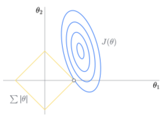
The Lasso method is a compression estimation method that replaces least squares. The basic idea of Lasso is to establish an L1 regularization model, which compresses some coefficients and sets some coefficients to zero during model establishment. Once the model training is complete, parameters with weights equal to 0 can be discarded, making the model simpler and effectively preventing overfitting. It is widely used for fitting and variable selection in the presence of multicollinearity data.
1.14 K-Nearest Neighbors (KNN)
The main difference between KNN for regression and classification lies in the decision-making method during prediction. When KNN performs classification prediction, it generally uses the majority vote method, i.e., it predicts the category that appears most among the K nearest samples in the training set. When KNN performs regression, it generally uses the average method, taking the average value of the outputs of the K nearest samples as the regression prediction value. However, their theories are the same.
1.15 Decision Tree
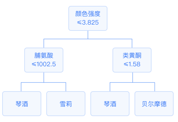
In a decision tree, each internal node represents a splitting problem: it specifies a test of a certain attribute of instances, which splits the samples reaching that node according to a specific attribute, and each subsequent branch of that node corresponds to a possible value of that attribute. The classification tree leaf node contains samples, and its output variable’s mode is the classification result. The regression tree leaf node contains samples, and its output variable’s mean is the prediction result.
1.16 BP Neural Network
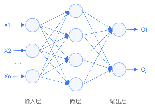
The BP neural network is a multilayer feedforward network trained by the error backpropagation algorithm, and it is one of the most widely used neural network models today. The learning rule of the BP neural network uses the steepest descent method to continuously adjust the network’s weights and thresholds through backpropagation, minimizing the network’s classification error rate (minimizing the sum of squared errors).
The BP neural network is a multilayer feedforward neural network characterized by: signals propagate forward while errors propagate backward. Specifically, for a neural network model with only one hidden layer:
The process of the BP neural network is mainly divided into two stages: the first stage is the forward propagation of signals from the input layer through the hidden layer to the output layer; the second stage is the backward propagation of errors from the output layer to the hidden layer and finally to the input layer, sequentially adjusting the weights and biases from the hidden layer to the output layer and from the input layer to the hidden layer.
1.17 Support Vector Machine (SVM)
Support Vector Machine Regression (SVR) maps data into a high-dimensional feature space using nonlinear mapping, such that the independent and dependent variables have good linear regression characteristics in the high-dimensional feature space, and fitting is performed in that feature space before returning to the original space.
Support Vector Machine Classification (SVM) is a type of generalized linear classifier that performs binary classification on data using supervised learning, with its decision boundary being the maximum margin hyperplane solved from the learning samples.
1.18 Naive Bayes
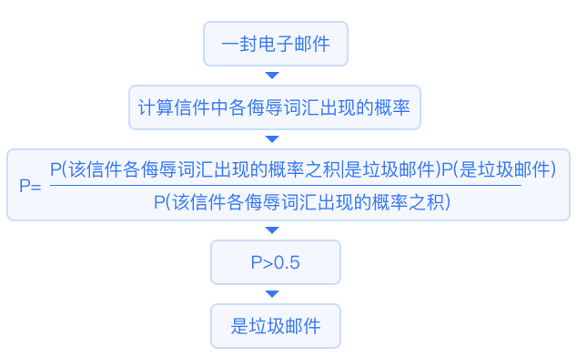
Given the premise of one event occurring, calculate the probability of another event occurring – we will use Bayes’ theorem. Assuming the prior knowledge is d, to calculate the probability that our hypothesis h is true, we will use the following Bayes’ theorem:
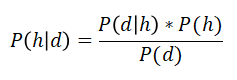
This algorithm assumes that all variables are independent of each other.
1.2 Ensemble Learning
Ensemble learning is a method that combines the results of different learning models (such as classifiers) to further improve accuracy through voting or averaging. Generally, voting is used for classification problems, and averaging is used for regression problems. This approach is derived from the idea of “many hands make light work.”
There are three main types of ensemble algorithms: Bagging, Boosting, and Stacking. This article will not discuss stacking.

-
Boosting
1.21 GBDT
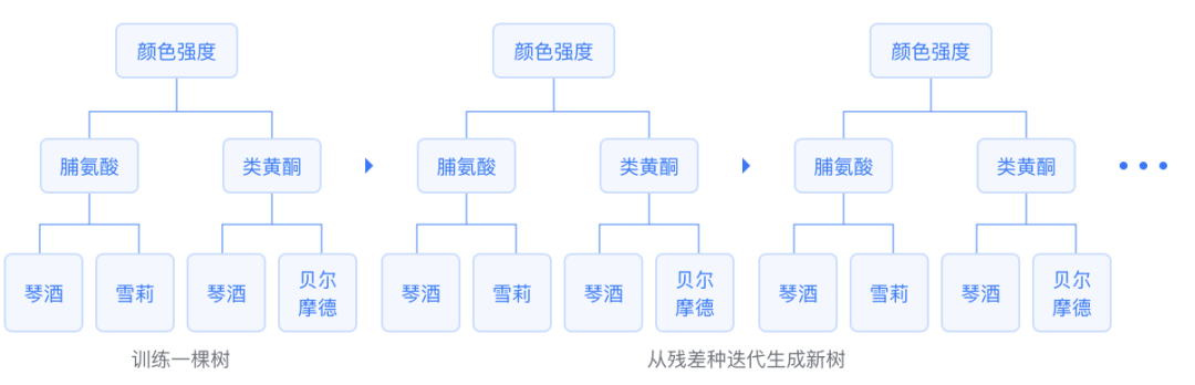
GBDT is a Boosting algorithm with CART regression trees as the base learner. It is an additive model that serially trains a set of CART regression trees, and finally sums the predictions of all regression trees to obtain a strong learner. Each new tree fits the negative gradient direction of the current loss function. The final output is the sum of this set of regression trees, directly yielding regression results or applying the sigmoid or softmax function to obtain binary or multi-class results.
1.22 AdaBoost
AdaBoost gives a high weight to learners with low error rates and a low weight to learners with high error rates, combining weak learners with their corresponding weights to generate a strong learner. The difference in algorithms for regression and classification problems lies in the way error rates are calculated; classification problems generally use a 0/1 loss function, while regression problems typically use a squared loss function or a linear loss function.
1.23 XGBoost
XGBoost stands for