Click on the above“Beginner’s Guide to Vision” to select “Star” or “Pin”
Heavyweight content delivered first timeFrom | Zhihu Author | Jixing
Link | https://zhuanlan.zhihu.com/p/147885624
Editor | Deep Learning Matters WeChat Official Account

Introduction
In recent years, with the tremendous breakthroughs in image recognition achieved by deep learning (represented by the high-precision AlexNet image recognition network proposed by AI pioneer Geoffry Hinton in 2012), a research boom based on neural networks has emerged. So far, image processing has become an important research area in deep learning, with almost all deep learning frameworks supporting image processing tools. The current applications of deep learning in image processing can be divided into three aspects: image processing (basic image transformations), image recognition (mainly neural network-based image feature extraction), and image generation (represented by neural style transfer). The first part of this article introduces common techniques for image processing in deep learning, the second part briefly analyzes mainstream applications of image processing in deep learning, and finally, a brief summary of the content of this article is provided.
I. Common Techniques for Image Processing in Deep Learning
Currently, almost all deep learning frameworks support image processing toolkits, including Tensorflow developed by Google and Microsoft’s CNTK. Using the simple-to-operate Keras frontend and Tensorflow backend development framework as an example, we introduce common operational techniques in image processing:
1. Data Augmentation:
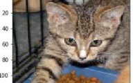
The three elements that restrict the development of deep learning are algorithm, computing power, and data. Among them, the performance of the algorithm is determined by the design method, and the key to computing power supply lies in the performance of hardware processors. When the algorithm and computing power are the same, the amount of data directly determines the final performance of the model. When performing image recognition, it is common to encounter overfitting of the output curve due to insufficient original images, making it impossible to train a model that generalizes to new image sets. Data augmentation generates more training images based on the currently known image dataset, specifically realized by using various random transformations that can generate credible images to increase the number of original images. The comparison results before and after data augmentation are shown in Figure 1:
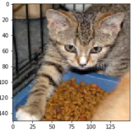
Figure 1a Original Image
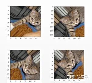
Figure 1b Image After Data Augmentation
Figure 1 Data Augmentation on Image
The key code is as follows (defining operations for augmented data, including scaling, shifting, and rotation):
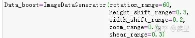
As can be seen from the comparison, data augmentation essentially expands the number of images without changing the feature content of the original images (for example, the key objects in the above image: cat, iron cage, food), thus avoiding the model’s overfitting and poor generalization caused by insufficient images, especially effective when training on small image datasets.
2. Image Denoising:
Real-world images can easily degrade in quality due to transmission fluctuations and interference from external noise during propagation. Image denoising refers to filtering out the interference information contained in the image while retaining useful information. Common denoising methods include non-local means filtering algorithm, Gaussian filtering algorithm, and convolutional neural networks that adaptively filter noise. A brief introduction is as follows:
1.2.1 Non-Local Means Filtering Algorithm.
The denoising principle of the non-local means filtering algorithm is as follows: the pixel setting in the image is determined by weighting it with surrounding pixels, meaning that the pixel setting of a certain point in the image relates to the weight setting of its surrounding pixels. The specific principle is shown in the following formula:
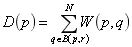
In the formula,  represents
  the weight of the pixel at the
  position, and
  represents the selection of pixels around the
  within a radius of
  pixels as weighted references.
  and
and  represent the statistical size of the pixel weights around the pixel point and the weighted sum of the pixel point affected by the surrounding pixels within the radius.
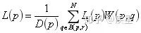
By adding noise to the original image, randomly setting 3000 pixels to white (RGB values all 255), it can be seen that the image with added noise adds many noise spots compared to the original image, as shown in Figure 2:
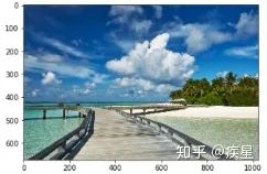
Figure 2a Original Beach Background Image
Figure 2b Background Image with Added Noise
Figure 2 Adding Random White Pixels to the Original Background Image to Simulate Actual Noise Interference
Then, using the built-in non-local means noise filtering algorithm of OpenCV to filter out the image noise, the result is shown in Figure 3:
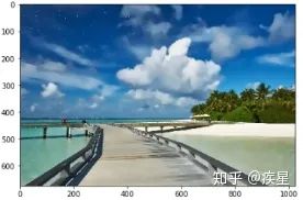
Figure 3 Background Image Obtained After Non-Local Means Noise Filtering
Observing the images before and after filtering with the non-local means noise algorithm, it can be seen that the white noise spots in the filtered image are significantly reduced, and the quality of the image is effectively improved, which is beneficial for subsequent encoding processing and transmission.
1.2.2 Denoising Neural Network.
Denoising neural networks are usually based on CNN (Convolutional Neural Network). Its essence is: using a denoising model trained on a noise-free image dataset to filter out noise information contained in the predicted image. The most common MNIST handwritten image library in image recognition is used as the training set, which contains 60,000 training images and 10,000 test images, each of size 28*28, classified into handwritten numbers 0-9. The MNIST database is built into Keras. The structure of the denoising neural network is shown in Figure 4:
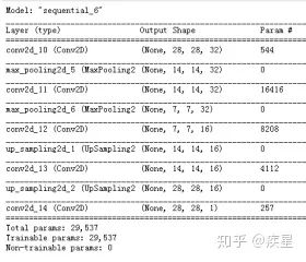
Figure 4 Simple Structure of Denoising Neural Network
Using the denoising neural network to denoise images with added noise from the MNIST image library, the comparison results before and after denoising are shown in Figures 5 and 6, where the subscripted Noise corresponds to Filter:
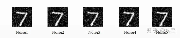
Figure 5 Adding Noise to the Original Image
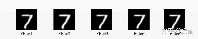 Figure 6 Using Denoising Neural Network to Filter Out Noise
Observing the images before and after denoising, it can be seen that the denoising neural network achieves the filtering of unnecessary noise information from the MNIST handwritten image set through feature extraction and supervised learning, making it a simple and commonly used image denoiser.
1.2.3 Image Super Resolution Reconstruction (SR, Super Resolution).
SR is a classic application in image processing and an important technology in the field of image enhancement. Its basic idea is to reconstruct a high-resolution image by extracting features from a low-resolution original image. According to the types and numbers of reference low-resolution images, it can be mainly divided into the following two types:
1. Image SR
The characteristic is that when reconstructing the image, there are few original low-resolution images available for reference, typically relying only on the current low-resolution image, also known as single image super resolution (SISR).
2. Video SR
The characteristic is that reconstructing the image requires referencing multiple different original low-resolution images, also known as multi-frame super resolution (MFSR). Typically, MFSR has higher reconstruction quality and more feature matching compared to SISR, at the cost of more computational resource consumption.
The quality of SR reconstruction can be evaluated by image quality assessment reference standards PSNR and SSIM. The higher the PSNR and SSIM values, the closer the reconstructed image pixel values are to the standard values. Among them, PSNR is defined as follows (MSE represents the mean squared error in image assessment):
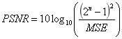
Where MSE is defined as follows:
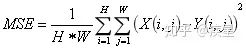
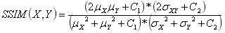
SSIM is simplified as follows (where represents  mean,
mean,  represents the mean square error):
In recent years, image super-resolution reconstruction technology has gradually become a research hotspot in the field of deep learning, with structures such as SRCNN (Super-Resolution Convolutional Neural Network) and FSRCNN (Fast Super-Resolution Convolutional Neural Network) emerging one after another. The following is a brief introduction:
1. SRCNN
SRCNN is an Image SR reconstruction network proposed by The Chinese University of Hong Kong in 2014. The core structure uses CNN to extract and map features from the original low-resolution image, ultimately completing the reconstruction of the high-resolution image. Its essence is to use deep learning neural networks to implement sparse autoencoders. The core structure of the SRCNN network is shown in Figure 7:
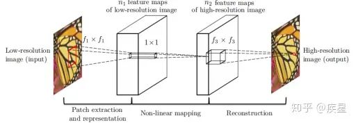
Figure 7 Structure Diagram of SRCNN Network
As shown in Figure 7, the process of the SRCNN network completing image super-resolution transformation is divided into three parts: first, the original low-resolution image is dimensionally expanded through interpolation, aiming to ensure that the input image to the network is the same size as the target image; then, the expanded original image is fitted through a convolutional network to extract features, completing the mapping from low-resolution feature maps to high-resolution feature maps. The CNN feature extraction network is the key structure of the SRCNN network, and the feature extraction network used in this article is a 3-layer stacked CNN; finally, based on the obtained high-resolution image features, the target image is reconstructed by combining dimensions and content, outputting the generated high-resolution image.
Comparing the SRCNN network with similar algorithms for high-resolution image reconstruction, the results are shown in Figure 8:
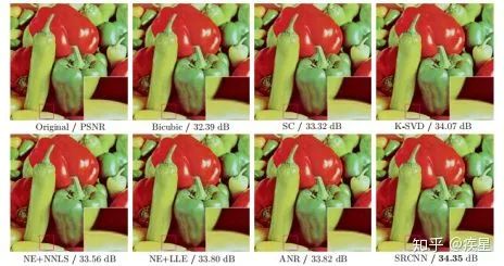
Figure 8a High-Resolution Image Reconstruction Using Different Super Resolution Methods
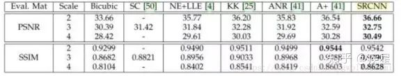
Figure 8b PSNR and SSIM Standard Evaluation of Common Super Resolution Reconstruction Methods
Figure 8 Performance Comparison of SRCNN Network and Traditional Methods
As shown in Figure 8, under the same conditions, the SSIM and PSNR values of the SRCNN network are mostly superior to those of traditional algorithms, indicating that the encoding quality of the SRCNN network is improved compared to traditional algorithms. Compared with traditional super-resolution algorithms, the SRCNN network has advantages such as simple structural principles and high reconstruction quality, but its disadvantage is a relatively low image transformation reconstruction speed.
2. FSRCNN
The FSRCNN network was also proposed by the SRCNN development team, aiming to improve the low image transformation speed of the SRCNN network. The modified network significantly improves the image transformation speed compared to the SRCNN network, with a slight improvement in image reconstruction quality. The changes made to the FSRCNN network compared to the SRCNN network are summarized as follows:
On dimensional transformation: The original SRCNN network performs interpolation transformation on the image from the moment it enters the network to complete the dimensional expansion to match the target image dimensions. This increases the tensor dimensions added at the beginning of the network, participating in all transformation operations between endpoints, greatly increasing the network’s computational complexity and operational overhead. The improved FSRCNN network places the dimensional expansion structure at the end of the network, avoiding unnecessary computational consumption introduced within the network, thus improving the image transformation speed.
On the computational structure: FSRCNN improves the nonlinear mapping method in feature mapping and reduces the convolution kernel dimensions during convolution operations, resulting in a significant reduction in the number of parameters for network operations and feature extraction, greatly enhancing the efficiency of high-resolution reconstruction. Due to changes in the internal structure of the network, the image quality reconstructed by FSRCNN is slightly improved compared to SRCNN. The comparison results between FSRCNN and SRCNN are shown in Figure 9, where the improved FSRCNN network shows improvements in both encoding quality and efficiency compared to the traditional SRCNN network.
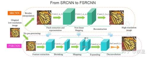
Figure 9a Comparison of Structures Between SRCNN and FSRCNN
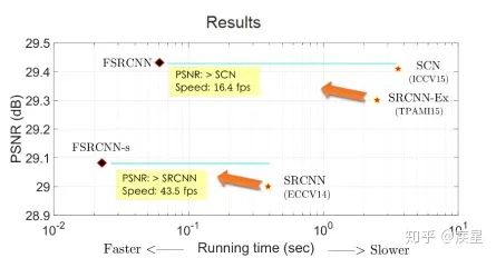
Figure 9b Comparison of Quality and Efficiency Between FSRCNN and SRCNN
II. Applications of Image Processing in Deep Learning
The current applications and developments of deep learning in image processing can be summarized into three aspects: image transformation, image recognition, and image generation, which are introduced from these three aspects:
2.1. Image Transformation
Refers to the routine operations performed on images, including simple operations such as image scaling, copying, etc., and common operations mentioned above such as denoising and enhancing super-resolution, with the aim of improving image quality to obtain the desired target image. Overall, image transformations performed by deep learning rely on the powerful functions of built-in tools, allowing users to learn the corresponding image processing tools based on different needs, which will not be elaborated here.
2.2. Image Recognition
Computer vision (CV) has become an important development direction in the field of deep learning, with the main content of CV being object recognition, and images as common objects in life have always been a research hotspot in CV. The typical method for image recognition using deep learning is to construct a neural network with the recognition object as the image, achieving high accuracy in image recognition with low computational resource consumption.
A brief introduction to using neural networks for image recognition is provided, taking the cat-dog image dataset provided by the Kaggle competition in 2013 as an example, constructing the image recognition neural network shown in Figure 10:
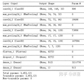
Figure 10 Simple Cat-Dog Image Recognition Neural Network
Setting the number of training epochs to 50, classifying 4000 cat-dog images, obtaining the trend of loss and accuracy during the training process of the image recognition network, as shown in Figure 11:
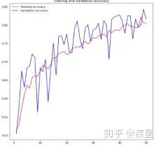
Figure a Accuracy Change During Image Recognition Process
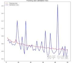
Figure b Loss Change During Image Recognition
Figure 11 Recognition Results of Cat-Dog Dataset Constructed by Image Recognition Network
As can be seen from Figure 11, the constructed simple image recognition network achieves over 80% recognition accuracy on the target image set after 50 iterations. Although there is overfitting during the recognition process, and the recognition accuracy is not satisfactory, the results prove the simplicity and feasibility of neural networks for image recognition. The negative impact of image overfitting can be reduced by methods such as reducing the number of network parameters (data weakening, etc.) and increasing the number of training images, while the recognition accuracy of the target images can be improved by methods such as adding pre-trained models.
Currently, high-precision image recognition constructed by neural networks has been widely applied in smart fields such as facial recognition, and relevant examples can be found online for further understanding. This article will not elaborate on it.
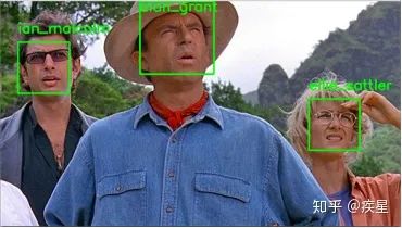
Figure 12 Results of Facial Recognition Using Neural Networks
2.3. Image Generation
Image generation refers to the process of learning features from known images and then combining them to generate new images. Unlike high-resolution reconstruction of images, image generation typically requires learning features of different images and combining them, with the generated images being a combination of all learned image features. Common applications of image generation include neural style transfer, Google’s Deep Dream algorithm, and variational autoencoders, which are introduced as follows:
2.3.1 Deep Dream
First released by Google in the summer of 2015, implemented using the early common Caffe architecture. Due to the algorithmically psychedelic illusion artifacts generated, it caused a sensation. A significant feature of images generated by Deep Dream is the abundance of bird feathers and dog eyes, as the original image library learned by DeepDream contains many samples of birds and dogs from ImageNet (a large open-source database commonly used for pre-training model weight training).
Deep Dream follows the same thought process as traditional convolutional neural network visualization, both performing gradient ascent on the input of the convolutional neural network to visualize a certain filter close to the network output; the difference is that the Deep Dream algorithm directly extracts features from existing images and attempts to maximize the activation of all layers in the neural network. Using the Deep Dream algorithm, feature transfer on known images is performed in the Keras framework, and the results are shown in Figure 13, where the images generated by Deep Dream add many features (mainly bird feather ripples and dog eyes) compared to the original images:
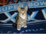
Figure 13a Original Cat Image
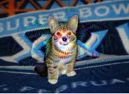
Figure 13b Deep Dream Cat Image

Figure 13c Original Dog Image
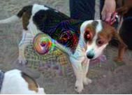
Figure 13d Deep Dream Dog Image
Figure 13 Images Generated Using Deep Dream Algorithm
2.3.2 Neural Style Transfer (NST)
Neural style transfer refers to applying the style of a reference image to a target image while preserving the content of the target image. Style refers to the textures, colors, and visual patterns of different spatial scales in the image, while content refers to the high-level macro structure of the image.
The idea of implementing neural style transfer is the same as that of ordinary deep learning methods, both aiming to minimize the defined loss. Unlike conventional deep learning algorithms, the loss function of neural style transfer is mathematically defined in relation to the content and style of the image. The specific definition is shown in the following formula:

In the formula,  represents the loss defined between the reference image and the generated image, composed of
  style loss and
  content loss.
  and
and  are defined as style loss function and content loss function, respectively.
The content loss function is calculated based on the differences between the reference image and the generated image using the activations of the network closer to the top layer, as the selected network layers are closer to the output end, it can be considered that the differences obtained by the content loss function represent the differences in more global abstract image content between the target image and the generated image.
The style loss function, on the other hand, uses multiple layers of the neural network, aiming to ensure that the activations of each layer in the neural network maintain similar internal relationships between the style reference image and the generated image. Unlike the content loss function, which focuses on more global and primary image content, the style loss function needs to maintain similar mutual relationships at both higher and lower layers of the network, fundamentally ensuring that the style of the reference image does not change during feature extraction.
The process of implementing neural style transfer is divided into three steps:
1. Load the pre-trained network, creating a neural network that can simultaneously compute the activations of the style reference image, target image, and generated image.
2. Use the corresponding layer activations computed from the three images to define the content loss and style loss, obtaining the overall loss function.
3. Set up batch gradient descent to minimize the target loss.
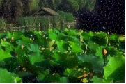
Using Keras’s built-in VGG19 pre-trained model to implement neural style transfer, the target is to achieve the original neural style transfer algorithm proposed in 2015, and the transfer results are shown in Figure 13:

Original Image of Starry Sky

Original Image of Lotus Pond
Figure 14a Original Images for Implementing Neural Style Transfer
Starry Lotus Pond
Lotus Pond with Stars
Figure 14b Transfer Results Obtained by Swapping Reference and Target Images
Figure 14 Implementing Original Neural Style Transfer Using Keras
Observing Figure 13, it can be seen that the transfer neural network successfully completed the style transfer from the reference image to the target image while preserving the content of the target image. Using the starry sky and lotus pond as reference objects, the resulting target images are the starry lotus pond and lotus pond with stars. By reasonably selecting the original images and defining the transfer parameters, a series of stunning images can be generated.
2.3.3 Variational Autoencoder (VAE)
The variational autoencoder was first proposed by Kingma and Welling in December 2013. It is a type of autoencoder built using generative models in deep learning, characterized by combining deep learning ideas with Bayesian inference to complete the encoding mapping of input targets to low-dimensional vector space and the decoding to high-dimensional vector space. Classic image autoencoders first use an encoder module to encode the received image, mapping it to a latent vector space composed of image features; then, the decoder module decodes it into an output of the same dimension as the target image. The workflow of classic autoencoders is shown in Figure 15.
In practice, classic autoencoders often lead to discontinuous generated images due to the lack of well-structured latent learning space, failing to efficiently extract features from the original training images. Variational autoencoders change the encoding and decoding methods based on classic autoencoders, obtaining a continuous and highly structured latent space. VAE does not compress the input image into a fixed code in the latent space but converts the image into statistical distribution parameters (mean and variance). Then, VAE randomly samples an element from the distribution using these two parameters and decodes it back to the original input. This randomness enhances its robustness and forces any position in the latent space to correspond to meaningful representations, meaning that every point sampled in the latent space can be decoded into valid output. The workflow of the variational autoencoder is shown in Figure 16.
Image variational autoencoders, like general deep learning models, use images of the same type and size as the input to train the model, completing feature extraction of input images and automatic reconstruction generation of target images. Specific features can be constrained by specifying the output of the encoder.
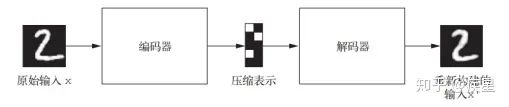
Figure 15 Workflow Diagram of Classic Autoencoder
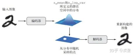
Figure 16 Workflow of Variational Autoencoder (z_mean and z_log_var represent the mean and variance of the latent image mapped by the encoder)
Using the MNIST dataset as the training dataset for the variational autoencoder, the generated images are shown in Figure 17:
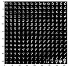
Figure 17 Handwritten Digit Images Generated by VAE
2.3.4 Generative Adversarial Networks (GAN)
GAN was proposed by Goodfellow et al. in 2014 and can replace VAE to learn the latent space of images, generating images that are statistically indistinguishable from real images, thus producing quite realistic synthetic images.
The GAN structure consists of a generator network and a discriminator network, both trained to outsmart each other. The generator network takes a random vector (a random point in the latent space) as input and decodes it into a synthetic image. The discriminator network, also known as the adversary network, takes an image (either real or synthetic) as input and predicts whether the image comes from the training set or the generator network. The goal of training the generator network is to enable it to deceive the discriminator network, so as training progresses, it can gradually generate increasingly realistic images, which appear indistinguishable from real images, to the point where the discriminator network cannot tell the difference. The workflow of GAN is shown in Figure 18:
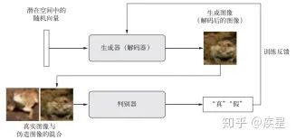
Figure 18 Training Process of GAN Network
The process of training GAN and adjusting its implementation is very challenging. This article will not elaborate on this; readers can refer to relevant materials for further understanding. The images of faces generated using GAN are shown in Figure 19:
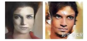
Figure 19 Images Generated by GAN on Face Image Dataset
III. Summary
This article first introduced common techniques for image processing in the field of deep learning, including data augmentation, image denoising, and image high-resolution reconstruction technology (SR, Super Resolution) in the field of image enhancement. Data augmentation can generate more training images with similar content and style based on original images, effectively addressing the issue of curve overfitting caused by insufficient training images; the representative techniques for image denoising are common Gaussian filtering algorithms and denoising neural networks, which share the common feature of effectively filtering interference fluctuations encountered during image transmission, beneficial for subsequent image processing; image high-resolution reconstruction is a significant representative in the field of image enhancement, with the basic idea being to extract features from the original low-resolution images, transforming and mapping them to obtain high-resolution images. This technology not only preserves the content and style of the original images (the effective information of the images) but also improves the quality of the transformed images.
The second part of this article briefly analyzes the main applications of deep learning technology in the field of image processing, categorized into three areas based on different functions: image transformation, image recognition, and image generation. Image transformation is the simplest and most basic operation in image processing; image recognition is an important branch of research in computer vision, aiming to enhance the recognition accuracy and efficiency of deep learning image recognition networks, with practical applications in facial recognition and remote sensing image recognition; finally, a brief overview of several branches of image generation applications is provided, including neural style transfer (NST) and variational autoencoders (VAE). Deep Dream can be regarded as a neural style transfer network trained on ImageNet, whose common feature is to extract and combine content and style from reference images to generate various target images as required. Another important branch in the field of image generation is Generative Adversarial Networks (GAN), which can generate target images that are very similar to the original images; interested readers can explore further.
The field of image processing is an important research branch of deep learning and machine vision, and it is believed that it will thrive in the future. The images and code involved in this article can be downloaded and accessed at github.com/asbfighting/.
Good News!
Beginner’s Guide to Vision Knowledge Circle
Is now open to the public👇👇👇
Download 1: OpenCV-Contrib Extension Module Chinese Version Tutorial
Reply "Extension Module Chinese Tutorial" in the "Beginner's Guide to Vision" WeChat official account to download the first OpenCV extension module tutorial in Chinese, covering over twenty chapters including extension module installation, SFM algorithms, stereo vision, object tracking, biological vision, super-resolution processing, etc.

Download 2: Python Vision Practical Project 52 Lectures
Reply "Python Vision Practical Project" in the "Beginner's Guide to Vision" WeChat official account to download 31 visual practical projects including image segmentation, mask detection, lane line detection, vehicle counting, eyeliner addition, license plate recognition, character recognition, emotion detection, text content extraction, facial recognition, etc., to help quickly learn computer vision.

Download 3: OpenCV Practical Project 20 Lectures
Reply "OpenCV Practical Project 20 Lectures" in the "Beginner's Guide to Vision" WeChat official account to download 20 practical projects based on OpenCV, achieving advanced learning in OpenCV.

Group Discussion

Welcome to join the reader group of the WeChat official account to communicate with peers. Currently, there are WeChat groups for SLAM, 3D vision, sensors, autonomous driving, computational photography, detection, segmentation, recognition, medical imaging, GAN, algorithm competitions, etc. (which will gradually be subdivided later). Please scan the WeChat ID below to join the group, and note: "Nickname + School/Company + Research Direction", for example: "Zhang San + Shanghai Jiao Tong University + Vision SLAM". Please follow the format for notes, otherwise, it will not be approved. After successful addition, invitations to relevant WeChat groups will be sent based on research direction. Please do not send advertisements in the group, otherwise you will be removed from the group. Thank you for your understanding.~