
Source: You Er's Cabin - New Machine Vision

This article is about 7000 words long and is recommended to read in 14 minutes.
This article shares a piece about clustering: 10 clustering algorithms and their Python code.
Clustering or cluster analysis is an unsupervised learning problem. It is commonly used as a data analysis technique to discover interesting patterns in data, such as customer groups based on their behavior.
There are many clustering algorithms to choose from, and there is no single best clustering algorithm for all situations. Instead, it is best to explore a range of clustering algorithms along with different configurations for each algorithm. In this tutorial, you will discover how to install and use top clustering algorithms in Python.
By the end of this tutorial, you will know:
-
Clustering is an unsupervised problem that looks for natural groups in the feature space of input data.
-
For all datasets, there are many different clustering algorithms and no single best method.
-
How to implement, adapt, and use top clustering algorithms in Python using the Scikit-learn machine learning library.
Tutorial Overview
This tutorial is divided into three parts:
1. Clustering
2. Clustering Algorithms
3. Examples of Clustering Algorithms
1. Library Installation
2. Clustering Dataset
3. Examples
3.1 Affinity Propagation
3.2 Agglomerative Clustering
3.3 BIRCH
3.4 DBSCAN
3.5 K-Means
3.6 Mini-Batch K-Means
3.7 Mean Shift
3.8 OPTICS
3.9 Spectral Clustering
3.10 Gaussian Mixture Model
1. Clustering
Cluster analysis, or clustering, is an unsupervised machine learning task. It involves automatically discovering natural groupings in data. Unlike supervised learning (similar to predictive modeling), clustering algorithms only interpret the input data and find natural groups or clusters in the feature space.
Clustering techniques are suitable for cases where there are no classes to predict, but rather instances are divided into natural groups.
—Source: “Data Mining: Practical Machine Learning Tools and Techniques”, 2016.
Clusters are typically dense regions in the feature space where examples (observations or data rows) from the domain are closer to each other than to other clusters. Clusters can have a center (centroid) as samples or points in the feature space, and can have boundaries or extents.
These clusters may reflect some mechanism at work in the domain from which the instances are drawn, which causes certain instances to be more similar to each other than they are to the rest of the instances.
—Source: “Data Mining: Practical Machine Learning Tools and Techniques”, 2016.
Clustering can assist as a data analysis activity to gain more information about the problem domain, known as pattern discovery or knowledge discovery. For example:
-
The evolutionary tree can be thought of as the result of artificial cluster analysis;
-
Separating normal data from outliers or anomalies might be considered a clustering problem;
-
Separating clusters based on natural behavior is a clustering problem known as market segmentation.
Clustering can also serve as a type of feature engineering, where existing and new examples can be mapped and labeled as belonging to one of the clusters identified in the data. While there are indeed many clustering-specific quantitative measures, the evaluation of the identified clusters is subjective and may require domain experts. Typically, clustering algorithms are academically compared on artificially generated datasets against predefined clusters, which the pre-calculated methods will discover.
Clustering is an unsupervised learning technique, making it difficult to assess the quality of the output of any given method.
—Source: “Machine Learning: A Probabilistic Perspective”, 2012.
2. Clustering Algorithms
There are many types of clustering algorithms. Many algorithms use similarity or distance metrics between examples in the feature space to discover dense observation areas. Therefore, it is generally good practice to scale the data before using clustering algorithms.
At the core of all clustering analysis objectives is the concept of the degree of similarity (or dissimilarity) between the individual objects being clustered. Clustering methods attempt to define groups of objects based on the similarities provided to the objects.
—Source: “The Elements of Statistical Learning: Data Mining, Inference, and Prediction”, 2016
Some clustering algorithms require you to specify or guess the number of clusters to discover in the data, while others require specifying the minimum distance between observations, where examples can be considered “close” or “connected”. Therefore, clustering analysis is an iterative process in which the subjective evaluation of the identified clusters is fed back into changes in the algorithm configuration until the desired or appropriate results are achieved. The Scikit-learn library provides a set of different clustering algorithms to choose from. Below are 10 popular algorithms::
-
Affinity Propagation
-
Agglomerative Clustering
-
BIRCH
-
DBSCAN
-
K-Means
-
Mini-Batch K-Means
-
Mean Shift
-
OPTICS
-
Spectral Clustering
-
Gaussian Mixture
Each algorithm provides a different approach to tackling the challenge of discovering natural groups in data. There is no best clustering algorithm, nor is there a simple way to find the best algorithm for your data without using controlled experiments.
In this tutorial, we will review how to use each of these 10 popular clustering algorithms from the Scikit-learn library. These examples will provide a foundation for you to copy and paste examples and test the methods on your own data. We will not delve deeply into the theory of how the algorithms work, nor will we directly compare them. Let’s dive in.
3. Examples of Clustering Algorithms
In this section, we will review how to use 10 popular clustering algorithms in Scikit-learn, including an example of fitting a model and an example of visualizing the results. These examples are meant for you to copy and paste into your own projects and apply the methods to your own data.
1. Library Installation
First, let’s install the library. Do not skip this step, as you need to ensure you have the latest version installed. You can install the Scikit-learn library using the pip Python installer as follows:
sudo pip install scikit-learnNext, let’s confirm that the library is installed and that you are using a modern version. Run the following script to output the library version number.
# Check scikit-learn version
import sklearn
print(sklearn.__version__)
When you run this example, you should see the following version number or higher.
0.22.12. Clustering Dataset
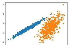
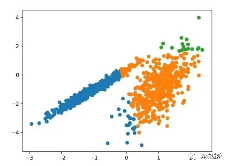
We will use the make_classification() function to create a test binary classification dataset. The dataset will have 1000 examples, with two input features for each class and one cluster. These clusters are visible in two dimensions, so we can plot the data with a scatter plot and color the points in the plot according to the specified clusters.
This will help to understand how well the clustering capability performs, at least on the test problem. The clusters in this test problem are based on multivariate Gaussian, and not all clustering algorithms can effectively identify these types of clusters. Therefore, the results in this tutorial should not be used as a basis for comparing general methods. Below is an example of creating and summarizing a synthetic clustering dataset.
# Create synthetic classification dataset
from numpy import where
from sklearn.datasets import make_classification
from matplotlib import pyplot
%matplotlib inline

# Define dataset
X, y = make_classification(n_samples=1000,
                            n_features=2,
                            n_informative=2,
                            n_redundant=0,
                            n_clusters_per_class=1,
                            random_state=4)

# Create scatter plot for samples of each class
for class_value in range(2):
    # Get row index for this class
    row_ix = where(y == class_value)
    # Create scatter for these samples
    pyplot.scatter(X[row_ix, 0], X[row_ix, 1])

# Show scatter plot
pyplot.show()
Running this example creates a synthetic clustering dataset, then creates a scatter plot of the input data where the points are colored according to class labels (idealized clusters). We can clearly see two distinct groups of data in two dimensions, and hope that an automatic clustering algorithm can detect these groupings.
Next, we can start looking at examples of clustering algorithms applied to this dataset. I have made some minimal attempts to tune each method to the dataset.
3. Examples
3.1 Affinity Propagation
Affinity Propagation involves finding a set of exemplars that best summarize the data.
We designed a method called “Affinity Propagation” that acts as an input measure of similarity between pairs of data points. Real-valued messages are exchanged between data points until a set of high-quality exemplars and corresponding clusters gradually emerge.
—Source: “Message Passing Between Data Points”, 2007.
It is implemented through the AffinityPropagation class, with the main configuration to tune being the “damping” set between 0.5 to 1, and possibly the “preference”. Below is a complete example.
# Affinity Propagation Clustering
from numpy import unique
from numpy import where
from sklearn.datasets import make_classification
from sklearn.cluster import AffinityPropagation
from matplotlib import pyplot
# Define dataset
X, _ = make_classification(n_samples=1000,
n_features=2,
n_informative=2,
n_redundant=0,
n_clusters_per_class=1,
random_state=4)
# Define model
model = AffinityPropagation(damping=0.9)
# Fit model
model.fit(X)
# Assign a cluster for each example
yhat = model.predict(X)
# Retrieve unique clusters
clusters = unique(yhat)
# Create scatter plot for samples of each cluster
for cluster in clusters:
# Get row index for this cluster
row_ix = where(yhat == cluster)
# Create scatter for these samples
pyplot.scatter(X[row_ix, 0], X[row_ix, 1])
# Show scatter plot
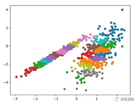
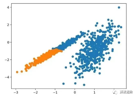
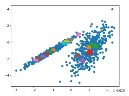
pyplot.show()Running this example fits the model on the training dataset and predicts the cluster for each example in the dataset, then creates a scatter plot colored by their assigned clusters. In this case, I was unable to achieve good results.
3.2 Agglomerative Clustering
Agglomerative clustering involves merging examples until the desired number of clusters is reached. It is part of a broader class of hierarchical clustering methods implemented through the AgglomerativeClustering class, with the main configuration being the “n_clusters” parameter, which is an estimate of the number of clusters in the data. Below is a complete example:
# Agglomerative Clustering
from numpy import unique
from numpy import where
from sklearn.datasets import make_classification
from sklearn.cluster import AgglomerativeClustering
from matplotlib import pyplot
# Define dataset
X, _ = make_classification(n_samples=1000,
n_features=2,
n_informative=2,
n_redundant=0,
n_clusters_per_class=1,
random_state=4)
# Define model
model = AgglomerativeClustering(n_clusters=2)
# Fit model and predict clusters
yhat = model.fit_predict(X)
# Retrieve unique clusters
clusters = unique(yhat)
# Create scatter plot for samples of each cluster
for cluster in clusters:
# Get row index for this cluster
row_ix = where(yhat == cluster)
# Create scatter for these samples
pyplot.scatter(X[row_ix, 0], X[row_ix, 1])
# Show scatter plot
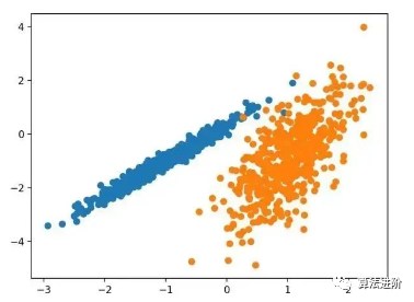
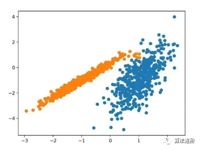
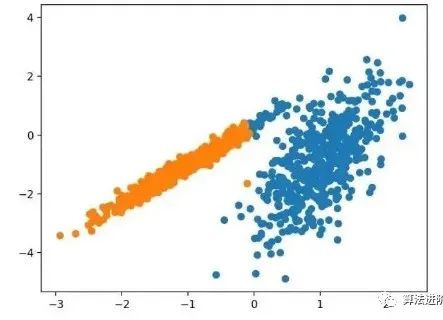
pyplot.show()Running this example fits the model on the training dataset and predicts the cluster for each example in the dataset, then creates a scatter plot colored by their assigned clusters. In this case, a reasonable grouping can be found.
3.3 BIRCH
BIRCH clustering (Balanced Iterative Reducing and Clustering using Hierarchies) involves constructing a tree structure from which cluster centroids are extracted.
BIRCH incrementally and dynamically clusters incoming multi-dimensional metric data points to try and produce the best quality clusters given available resources (i.e., memory and time constraints).
—Source: “BIRCH: An Efficient Data Clustering Method for Very Large Databases”, 1996
It is implemented through the Birch class, with the main configurations being the “threshold” and “n_clusters” hyperparameters, the latter providing an estimate of the number of clusters. Below is a complete example.
# BIRCH Clustering
from numpy import unique
from numpy import where
from sklearn.datasets import make_classification
from sklearn.cluster import Birch
from matplotlib import pyplot
# Define dataset
X, _ = make_classification(n_samples=1000,
n_features=2,
n_informative=2,
n_redundant=0,
n_clusters_per_class=1,
random_state=4)
# Define model
model = Birch(threshold=0.01, n_clusters=2)
# Fit model
model.fit(X)
# Assign a cluster for each example
yhat = model.predict(X)
# Retrieve unique clusters
clusters = unique(yhat)
# Create scatter plot for samples of each cluster
for cluster in clusters:
# Get row index for this cluster
row_ix = where(yhat == cluster)
# Create scatter for these samples
pyplot.scatter(X[row_ix, 0], X[row_ix, 1])
# Show scatter plot
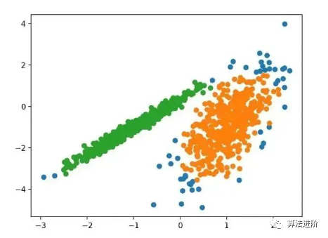
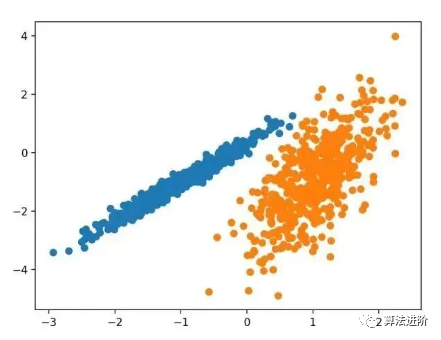
pyplot.show()Running this example fits the model on the training dataset and predicts the cluster for each example in the dataset, then creates a scatter plot colored by their assigned clusters. In this case, a good grouping can be found.
3.4 DBSCAN
DBSCAN clustering (Density-Based Spatial Clustering of Applications with Noise) involves searching for high-density regions in the domain and expanding the surrounding feature space regions into clusters.
…We propose a new clustering algorithm DBSCAN that relies on the density-based concept of cluster design to discover clusters of arbitrary shape. DBSCAN requires only one input parameter and supports the user in determining an appropriate value for it.
-Source: “A Density-Based Algorithm for Discovering Clusters in Large Spatial Databases with Noise”, 1996
It is implemented through the DBSCAN class, with the main configurations being the “eps” and “min_samples” hyperparameters.
Below is a complete example.
# DBSCAN Clustering
from numpy import unique
from numpy import where
from sklearn.datasets import make_classification
from sklearn.cluster import DBSCAN
from matplotlib import pyplot
# Define dataset
X, _ = make_classification(n_samples=1000,
n_features=2,
n_informative=2,
n_redundant=0,
n_clusters_per_class=1,
random_state=4)
# Define model
model = DBSCAN(eps=0.30, min_samples=9)
# Fit model and predict clusters
yhat = model.fit_predict(X)
# Retrieve unique clusters
clusters = unique(yhat)
# Create scatter plot for samples of each cluster
for cluster in clusters:
# Get row index for this cluster
row_ix = where(yhat == cluster)
# Create scatter for these samples
pyplot.scatter(X[row_ix, 0], X[row_ix, 1])
# Show scatter plot
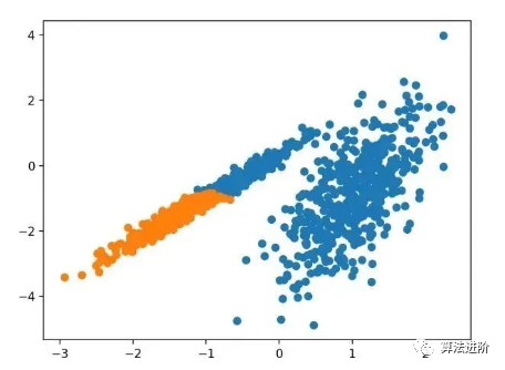
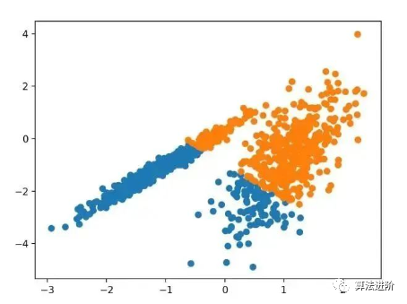
pyplot.show()Running this example fits the model on the training dataset and predicts the cluster for each example in the dataset, then creates a scatter plot colored by their assigned clusters. In this case, a reasonable grouping was found, although more tuning is needed.
3.5 K-Means
K-Means clustering can be the most common clustering algorithm and involves assigning examples to clusters in a way that minimizes variance within each cluster.
The main goal of this paper is to describe a process by which a sample divides an N-dimensional population into k sets. This process, called “K-Means,” appears to yield a fairly efficient partition in terms of within-class variance.
-Source: “Some Methods for Classification and Analysis of Multivariate Observations”, 1967
It is implemented through the KMeans class, with the main configuration to optimize being the “n_clusters” hyperparameter set to the estimated number of clusters in the data. Below is a complete example.
# K-Means Clustering
from numpy import unique
from numpy import where
from sklearn.datasets import make_classification
from sklearn.cluster import KMeans
from matplotlib import pyplot

# Define dataset
X, _ = make_classification(n_samples=1000,
                            n_features=2,
                            n_informative=2,
                            n_redundant=0,
                            n_clusters_per_class=1,
                            random_state=4)

# Define model
model = KMeans(n_clusters=2)

# Fit model
model.fit(X)

# Assign a cluster for each example
yhat = model.predict(X)

# Retrieve unique clusters
clusters = unique(yhat)

# Create scatter plot for samples of each cluster
for cluster in clusters:
    # Get row index for this cluster
    row_ix = where(yhat == cluster)
    # Create scatter for these samples
    pyplot.scatter(X[row_ix, 0], X[row_ix, 1])

# Show scatter plot
pyplot.show()
Running this example fits the model on the training dataset and predicts the cluster for each example in the dataset, then creates a scatter plot colored by their assigned clusters. In this case, a reasonable grouping was found, although the unequal variances in each dimension made this method less suitable for this dataset.
3.6 Mini-Batch K-Means
Mini-Batch K-Means is a modified version of K-Means that updates cluster centroids using small batches of samples instead of the entire dataset, which can speed up updates for large datasets and may be more robust to statistical noise.
…We propose a mini-batch optimization for k-means clustering. This reduces the computational cost by an order of magnitude compared to the classic batch algorithm while providing a better solution than online stochastic gradient descent. —Source: “Web-Scale K-Means Clustering”, 2010
It is implemented through the MiniBatchKMeans class, with the main configuration to optimize being the “n_clusters” hyperparameter set to the estimated number of clusters in the data. Below is a complete example.
# Mini-Batch K-Means Clustering
from numpy import unique
from numpy import where
from sklearn.datasets import make_classification
from sklearn.cluster import MiniBatchKMeans
from matplotlib import pyplot

# Define dataset
X, _ = make_classification(n_samples=1000,
                            n_features=2,
                            n_informative=2,
                            n_redundant=0,
                            n_clusters_per_class=1,
                            random_state=4)

# Define model
model = MiniBatchKMeans(n_clusters=2)

# Fit model
model.fit(X)

# Assign a cluster for each example
yhat = model.predict(X)

# Retrieve unique clusters
clusters = unique(yhat)

# Create scatter plot for samples of each cluster
for cluster in clusters:
    # Get row index for this cluster
    row_ix = where(yhat == cluster)
    # Create scatter for these samples
    pyplot.scatter(X[row_ix, 0], X[row_ix, 1])

# Show scatter plot
pyplot.show()
Running this example fits the model on the training dataset and predicts the cluster for each example in the dataset, then creates a scatter plot colored by their assigned clusters. In this case, a comparable result to the standard K-Means algorithm was found.
3.7 Mean Shift Clustering
Mean Shift clustering involves finding and adjusting centroids based on instance density in the feature space.
For discrete data, it has been shown that the recursive mean shift procedure converges to the nearest stationary point of the underlying density function, thus demonstrating its application in detecting density modes.
—Source: “Mean Shift: A Robust Method for Feature Space Analysis”, 2002
It is implemented through the MeanShift class, with the main configuration being the “bandwidth” hyperparameter. Below is a complete example.
# Mean Shift Clustering
from numpy import unique
from numpy import where
from sklearn.datasets import make_classification
from sklearn.cluster import MeanShift
from matplotlib import pyplot

# Define dataset
X, _ = make_classification(n_samples=1000,
                            n_features=2,
                            n_informative=2,
                            n_redundant=0,
                            n_clusters_per_class=1,
                            random_state=4)

# Define model
model = MeanShift()

# Fit model and predict clusters
yhat = model.fit_predict(X)

# Retrieve unique clusters
clusters = unique(yhat)

# Create scatter plot for samples of each cluster
for cluster in clusters:
    # Get row index for this cluster
    row_ix = where(yhat == cluster)
    # Create scatter for these samples
    pyplot.scatter(X[row_ix, 0], X[row_ix, 1])

# Show scatter plot
pyplot.show()
Running this example fits the model on the training dataset and predicts the cluster for each example in the dataset, then creates a scatter plot colored by their assigned clusters. In this case, a reasonable set of clusters can be found in the data.
3.8 OPTICS
OPTICS clustering (Ordering Points to Identify the Clustering Structure) is a modification of the aforementioned DBSCAN.
We introduce a new algorithm for cluster analysis that does not explicitly generate a clustering of a dataset; rather, it creates an augmented ordering of the database that represents its density-based clustering structure. This cluster ordering contains information equivalent to density clustering, which corresponds to a wide range of parameter settings.
—Source: “OPTICS: Ordering Points to Identify the Clustering Structure”, 1999
It is implemented through the OPTICS class, with the main configurations being the “eps” and “min_samples” hyperparameters. Below is a complete example.
# OPTICS Clustering
from numpy import unique
from numpy import where
from sklearn.datasets import make_classification
from sklearn.cluster import OPTICS
from matplotlib import pyplot

# Define dataset
X, _ = make_classification(n_samples=1000,
                            n_features=2,
                            n_informative=2,
                            n_redundant=0,
                            n_clusters_per_class=1,
                            random_state=4)

# Define model
model = OPTICS(eps=0.8, min_samples=10)

# Fit model and predict clusters
yhat = model.fit_predict(X)

# Retrieve unique clusters
clusters = unique(yhat)

# Create scatter plot for samples of each cluster
for cluster in clusters:
    # Get row index for this cluster
    row_ix = where(yhat == cluster)
    # Create scatter for these samples
    pyplot.scatter(X[row_ix, 0], X[row_ix, 1])

# Show scatter plot
pyplot.show()
Running this example fits the model on the training dataset and predicts the cluster for each example in the dataset, then creates a scatter plot colored by their assigned clusters. In this case, I was unable to achieve reasonable results on this dataset.
3.9 Spectral Clustering
Spectral clustering is a general class of clustering methods derived from linear algebra.
A promising alternative that has recently emerged in many fields is the use of spectral methods for clustering. Here, the top eigenvectors of a matrix derived from distances between points are used.
—Source: “A Survey of Spectral Clustering: Analysis and Algorithms”, 2002
It is implemented through the SpectralClustering class, and the main Spectral clustering is a general class of clustering methods derived from linear algebra. The main configuration to optimize is the “n_clusters” hyperparameter, which specifies the estimated number of clusters in the data. Below is a complete example.
# Spectral Clustering
from numpy import unique
from numpy import where
from sklearn.datasets import make_classification
from sklearn.cluster import SpectralClustering
from matplotlib import pyplot

# Define dataset
X, _ = make_classification(n_samples=1000,
                            n_features=2,
                            n_informative=2,
                            n_redundant=0,
                            n_clusters_per_class=1,
                            random_state=4)

# Define model
model = SpectralClustering(n_clusters=2)

# Fit model and predict clusters
yhat = model.fit_predict(X)

# Retrieve unique clusters
clusters = unique(yhat)

# Create scatter plot for samples of each cluster
for cluster in clusters:
    # Get row index for this cluster
    row_ix = where(yhat == cluster)
    # Create scatter for these samples
    pyplot.scatter(X[row_ix, 0], X[row_ix, 1])

# Show scatter plot
pyplot.show()
Running this example fits the model on the training dataset and predicts the cluster for each example in the dataset, then creates a scatter plot colored by their assigned clusters. In this case, reasonable clusters were found.
3.10 Gaussian Mixture Model
The Gaussian Mixture Model summarizes a multivariate probability density function, which is a mixture of Gaussian probability distributions. It is implemented through the GaussianMixture class, with the main configuration being the “n_clusters” hyperparameter used to specify the estimated number of clusters in the data. Below is a complete example.
# Gaussian Mixture Model
from numpy import unique
from numpy import where
from sklearn.datasets import make_classification
from sklearn.mixture import GaussianMixture
from matplotlib import pyplot

# Define dataset
X, _ = make_classification(n_samples=1000,
                            n_features=2,
                            n_informative=2,
                            n_redundant=0,
                            n_clusters_per_class=1,
                            random_state=4)

# Define model
model = GaussianMixture(n_components=2)

# Fit model
model.fit(X)

# Assign a cluster for each example
yhat = model.predict(X)

# Retrieve unique clusters
clusters = unique(yhat)

# Create scatter plot for samples of each cluster
for cluster in clusters:
    # Get row index for this cluster
    row_ix = where(yhat == cluster)
    # Create scatter for these samples
    pyplot.scatter(X[row_ix, 0], X[row_ix, 1])

# Show scatter plot
pyplot.show()
Running this example fits the model on the training dataset and predicts the cluster for each example in the dataset, then creates a scatter plot colored by their assigned clusters. In this case, we can see that the clusters are perfectly identified. This is not surprising as the dataset was generated as a mixture of Gaussians.
4. Summary
In this tutorial, you discovered how to install and use top clustering algorithms in Python. Specifically, you learned:
-
Clustering is an unsupervised problem of discovering natural groups in the feature space of input data.
-
There are many different clustering algorithms, and there is no single best method for all datasets.
-
How to implement, adapt, and use 10 top clustering algorithms in Python using the Scikit-learn machine learning library.
Editor: Yu Tengkai
Proofreader: Wang Xin