1. Introduction to Linear Regression
1.1 Origin of Regression
Francis Galton, a British biologist, studied the relationship between the heights of parents and their children. He concluded that if parents are taller than the average height of the population, their children tend to be shorter than their parents, moving closer to the average height of the population. Conversely, if parents are shorter than the average height, their children tend to be taller, again moving closer to the average height. This phenomenon was termed regression by Galton.
1.2 What is Linear Regression?
Regression analysis is a statistical tool that uses the relationship between two or more variables to predict another variable from one or several variables.
In regression analysis:
-
When there is only one independent variable, it is called simple linear regression, -
When there are multiple independent variables, it is called multiple linear regression,
Classification and regression both belong to supervised learning, and their distinction is as follows:
-
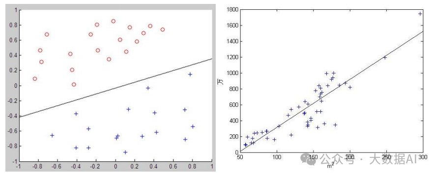
Classification: Qualitative output is called classification, or discrete variable prediction. For example, identifying normal emails vs. spam; identifying faces vs. non-faces in images; identifying normal behavior vs. fraud in credit.
-
Regression: Quantitative output is called regression, or continuous variable prediction. For example, predicting house prices given the area, location, and number of rooms.
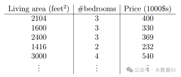
2. Relationship Between House Area, Number of Bedrooms, and House Prices
-
m: Size of the training data -
x: Input variable, is a vector -
y: Output variable, is a real number -
(x,y): A training instance -
: The i-th training instance, where i is a superscript, not an exponent -
n: Number of feature vectors, for example, in this instance it is 2
3. Model: Linear Regression
If we assume that the data in the training set is solved using linear regression, the hypothesis function is as follows:
the are the parameters (also called weights)
If we represent as a vector: , represented as a vector: , where, then
where indicates the parameter of . For a general problem, the formula is as follows:
4. Strategy: Least Squares Method
For a detailed introduction to the least squares method, please see the following articles:
-
Introduction to Least Squares -
Derivation and Proof of Ordinary Least Squares
4.1 Basic Idea
In simple terms, the idea of Least Mean Squares (LMS algorithm) is to minimize the sum of the squares of the distances between estimated points and observed points. Here, the square refers to using squares to measure the proximity of observed points to estimated points (in ancient Chinese, “squared” is referred to as “the square”), and the minimum indicates that the estimated values of the parameters should ensure that the sum of the squares of the distances between each observed point and the estimated point is minimized.
4.2 Role of Least Squares
It is used to obtain an optimal estimate of the parameters of the regression equation. In statistics, this estimation can fit the training samples well. Moreover, for new input samples, once the parameter estimates are available, they can be substituted into the formula to obtain the output of the input samples.
4.3 Cost Function
5. Algorithm: Gradient Descent
For a detailed introduction to the gradient descent algorithm, please see previous articles: Gradient Descent Method
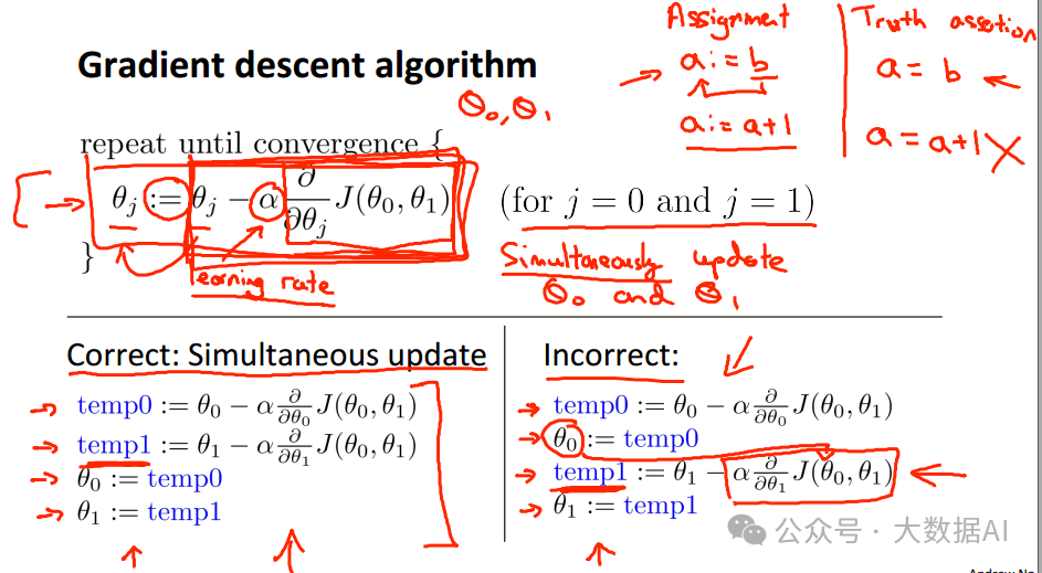
Using gradient descent to find parameters, the update rule is:
(This update is simultaneously performed for all values of j = 0, . . . , n.) Here, α is called the learning rate.
When there is only one training example, the formula for calculating the partial derivative is as follows:
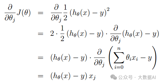
Substituting the above result into formula (6) gives:
or
Of course, formulas (7)/(8) are only the update rules for a single training instance. The rule is called the LMS update rule (LMS stands for “least mean squares”), and is also known as the Widrow-Hoff learning rule.
From formula (8), it can be seen that the value updated each time is proportional to the error term (error): . When the value of is large, the change value each time will also be large, and vice versa. When is already very small, it indicates that the fitting requirements have been met, and the value of will remain unchanged.
We’d derived the LMS rule for when there was only a single training example. There are two ways to modify this method for a training set of more than one example:
-
Batch Gradient Descent -
Stochastic Gradient Descent
5.1 Batch Gradient Descent
Algorithm:

It can be seen that each time the value of is updated, all samples in the sample set must be traversed to obtain the new , checking if it meets the threshold requirement. If it does, the iteration ends, and can be obtained based on this value; otherwise, it continues to iterate. It should be noted that although the gradient descent method is susceptible to the influence of local minima of the objective function, generally linear programming problems have only one minimum, so the gradient descent method can usually converge to the global minimum. For example, if is a quadratic convex function, the gradient descent method’s schematic diagram is:
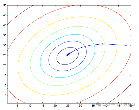
In the figure, the circles indicate the same value of the cost function, similar to geographical contour lines, starting from the outer circle and gradually iterating, ultimately converging to the global minimum.
The three-dimensional image in the above figure is:
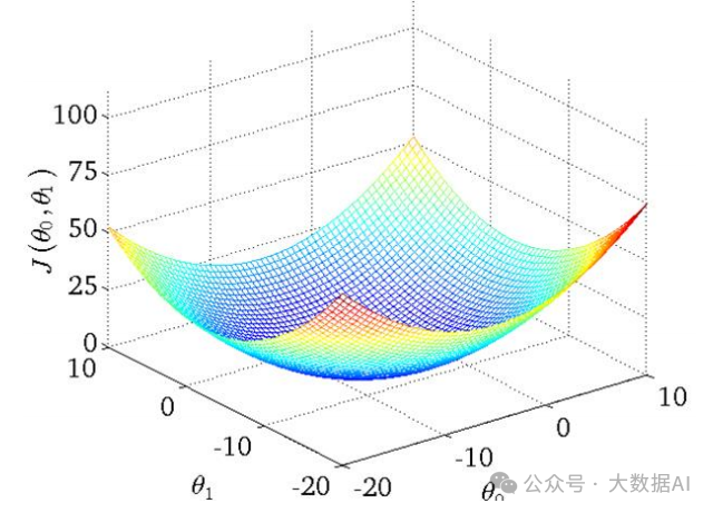
A more colloquial explanation is:
(1) The figure above actually looks like a bowl with a lowest point. The way to find this lowest point is to start from anywhere and move in the direction of the bowl’s descent until the lowest point is found.
(2) How to find the direction of descent from a certain point? Find the opposite direction of the derivative at that point. As shown in the following figure:
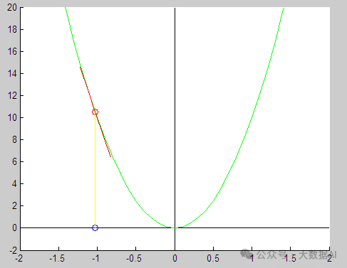
(3) As long as you move from any point in the opposite direction of the derivative, you will eventually reach the point that minimizes the function. (Note: The least squares method is a convex function, so the local optimum is also the global optimum.)
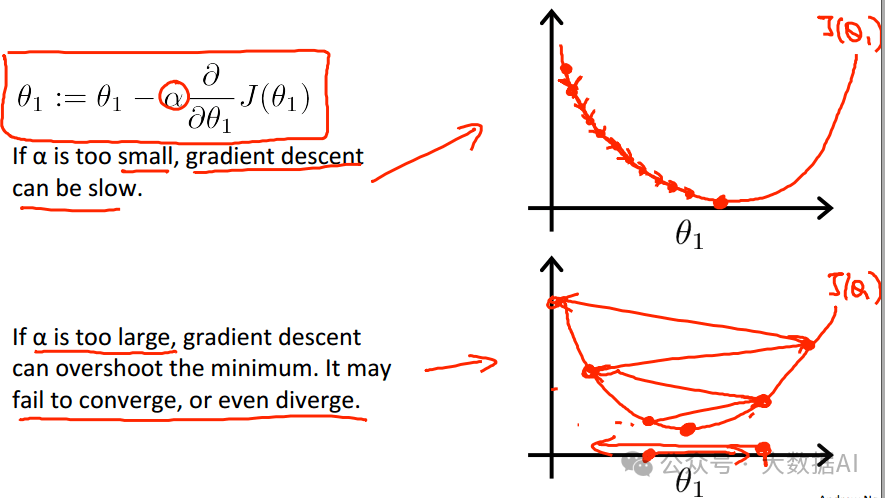
(4) is custom-defined, called the learning rate.
-
Setting it too small will cause slow convergence, taking many iterations. -
Setting it too large will cause oscillations beyond the optimum point, possibly never converging.
In general, programs will specify the maximum number of iterations and convergence conditions. If it can converge automatically, that’s great; if not, it will forcibly exit after a specified number of iterations. At this point, you need to adjust parameters or reconsider the assumed model!
The gradient descent algorithm can lead to local extreme points; a method to solve this is to randomly initialize and search for multiple optimal points, finding the final result among these optimal points.
Batch Gradient Descent Algorithm can become very slow when the amount of data is large, as each iteration requires traversing all data. To solve this problem, Stochastic Gradient Descent Algorithm can be used.
5.2 Stochastic Gradient Descent
Algorithm:
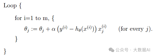
This method updates parameters without needing to traverse the entire dataset; each update only requires one sample. This algorithm can achieve very high performance, but it may lead to increased iterations and may not converge precisely to the optimal value. This method is called Stochastic Gradient Descent or Incremental Gradient Descent.
Note: It is necessary to update weights synchronously.
5.3 Batch Gradient Descent vs. Stochastic Gradient Descent
Batch Gradient Descent requires all samples in the sample set for each update; Stochastic Gradient Descent only requires one training sample for each update. Therefore, generally speaking, Stochastic Gradient Descent can make the objective function reach the minimum value faster (the addition of new samples may cause the objective function to suddenly increase, but it will decrease during the iteration). Thus, it hovers near the global minimum, but for practical applications, the error can fully meet the requirements. Moreover, for Batch Gradient Descent, if the sample set increases slightly, iteration must restart. For these reasons, when the training sample set is large, Stochastic Gradient Descent is generally used.
Additionally, there are two rules to judge convergence:
-
The change in parameters is very small after two iterations. -
The change in the objective function is very small after two iterations.
6. Normal Equation
The gradient descent algorithm is a method for finding the optimal solution of the objective function. For this problem, we can directly obtain the parameter values without iteration. This method is called the normal equation method.
The essence of the normal equation is the least squares method.
7. Gradient Descent vs. Normal Equation
| Gradient Descent | Normal Equation |
|---|---|
| Custom-defined | No need for definition |
| Requires N iterations to get the best w value | No looping required |
| Applicable when the number of features is very large | Calculating the transpose and inverse of the matrix is very large, making it slow when the number of features is high |
| Requires feature scaling | No need for feature scaling |
8. Feature Scaling
When there are multiple features, if the ranges of the features differ greatly, what impact and consequences will it have?
For example, continuing with the house price prediction example, now its features have increased: feature 1 is area, feature 2 is the number of rooms, and feature 3 is the age of the house. Clearly, the value ranges of these three features vary significantly.
-
Feature 1: Between 100 and 300 -
Feature 2: Between 2 and 5 -
Feature 3: Between 20 and 60 years
If no processing is done, then the influence of features 1 and 3 on the result will far exceed that of feature 2, which may distort the actual weight proportions that each feature should have in the final result.
Therefore, generally, when the value ranges of features differ too much, we use feature scaling methods to normalize feature values, ensuring that each feature’s value is within -1 to 1.
If the sizes between different variables are not on the same order of magnitude, feature scaling can significantly reduce the time needed to find the optimal solution;
The methods of feature scaling can be customized, commonly used methods include:
-
Rescaling: (X – mean(X))/(max – min) -
Mean normalization: (X-mean(X))/ std, where std is standard deviation
9. Common Questions
Question 1: If the step size is fixed, will it be too large when approaching the minimum point?
**Answer:** No. Because the effective step size is step size * slope value, and as you get closer to the minimum point, the slope approaches 0, making step size * slope smaller.
Question 2: How to choose the step size?
Answer: A step size that is too small will cause the cost function to converge slowly, while a step size that is too large may prevent convergence. You can try values like 0.1, 0.01, 0.001, etc., spaced by factors of 10 or 3, and observe the cost function’s change curve. If the curve decreases too gently, increase the step size; if the curve fluctuates greatly or does not converge, decrease the step size.
Question 3: Can stochastic gradient descent find the value that minimizes the cost function?
Answer: Not necessarily, but as the number of iterations increases, it will hover near the optimal solution, which is sufficient for us, as machine learning algorithms are not 100% accurate.
Question 4: Since there is a normal equation, why use gradient descent?
Answer: Because the normal equation involves matrix inversion operations, but this inverse matrix does not always exist, for example, when the number of samples is less than the number of features (i.e., m<n). Additionally, when the number of samples is very large, with many features, this creates a massive matrix, making direct solving impractical.