Approximately 3800 words, recommended reading time 6 minutes. This article introduces 10 nonlinear dimensionality reduction techniques in machine learning.
Dimensionality reduction means reducing the number of features in a dataset without losing too much information. Dimensionality reduction algorithms fall under the category of unsupervised learning, training algorithms with unlabeled data.
Although there are many types of dimensionality reduction methods, they can be classified into two main categories: linear and nonlinear.
Linear methods project data from high-dimensional space to low-dimensional space linearly (hence called linear projection). Examples include PCA and LDA.
Nonlinear methods provide a way to perform nonlinear dimensionality reduction (NLDR). We often use NLDR to discover the nonlinear structure of the original data. NLDR is useful when the original data cannot be linearly separated. In some cases, nonlinear dimensionality reduction is also referred to as manifold learning.
This article summarizes 10 commonly used nonlinear dimensionality reduction techniques to help you make selections in your daily work.
1. Kernel PCA
You may be familiar with normal PCA, which is a linear dimensionality reduction technique. Kernel PCA can be viewed as the nonlinear version of normal principal component analysis.
Both conventional PCA and kernel PCA can perform dimensionality reduction. However, kernel PCA can handle linearly inseparable data well. Therefore, the main purpose of the kernel PCA algorithm is to make linearly inseparable data linearly separable while reducing the dimensionality of the data!
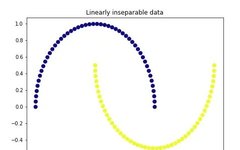
Let’s first create a very classic dataset:
import matplotlib.pyplot as plt plt.figure(figsize=[7, 5]) from sklearn.datasets import make_moons X, y = make_moons(n_samples=100, noise=None, random_state=0) plt.scatter(X[:, 0], X[:, 1], c=y, s=50, cmap='plasma') plt.title('Linearly inseparable data')
The two colors represent two classes that are linearly inseparable. It is impossible to draw a straight line to separate these two classes.
Let’s first use conventional PCA.
import numpy as np from sklearn.decomposition import PCA pca = PCA(n_components=1) X_pca = pca.fit_transform(X) plt.figure(figsize=[7, 5]) plt.scatter(X_pca[:, 0], np.zeros((100,1)), c=y, s=50, cmap='plasma') plt.title('First component after linear PCA') plt.xlabel('PC1')
As can be seen, these two classes are still linearly inseparable, now let’s try kernel PCA.
import numpy as np from sklearn.decomposition import KernelPCA kpca = KernelPCA(n_components=1, kernel='rbf', gamma=15) X_kpca = kpca.fit_transform(X) plt.figure(figsize=[7, 5]) plt.scatter(X_kpca[:, 0], np.zeros((100,1)), c=y, s=50, cmap='plasma') plt.axvline(x=0.0, linestyle='dashed', color='black', linewidth=1.2) plt.title('First component after kernel PCA') plt.xlabel('PC1')
These two classes have become linearly separable. The kernel PCA algorithm transforms data from one form to another using different kernels. Kernel PCA is a two-step process. First, the kernel function temporarily projects the original data into high-dimensional space, where the classes are linearly separable. Then, the algorithm projects that data back into the lower dimension specified by the n_components hyperparameter (the dimensions we want to retain).
There are four kernel options in sklearn: ‘linear’, ‘poly’, ‘rbf’, and ‘sigmoid’. If we specify the kernel as ‘linear’, normal PCA will be performed. Any other kernel will perform nonlinear PCA. The rbf (Radial Basis Function) kernel is the most commonly used.
2. Multidimensional Scaling (MDS)
Multidimensional scaling is another nonlinear dimensionality reduction technique that performs dimensionality reduction by preserving distances between high-dimensional and low-dimensional data points. For example, points that are close together in the original dimensions also appear closer in the low-dimensional form.
To use MDS in Scikit-learn, we can use the MDS() class.
from sklearn.manifold import MDS mds = MDS(n_components, metric) mds_transformed = mds.fit_transform(X)
The metric hyperparameter distinguishes between two types of MDS algorithms: metric and non-metric. If metric=True, metric MDS is performed. Otherwise, non-metric MDS is performed.
We will apply both types of MDS algorithms to the following nonlinear data.
import numpy as np from sklearn.manifold import MDS mds = MDS(n_components=1, metric=True) # Metric MDS X_mds = mds.fit_transform(X) plt.figure(figsize=[7, 5]) plt.scatter(X_mds[:, 0], np.zeros((100,1)), c=y, s=50, cmap='plasma') plt.title('Metric MDS') plt.xlabel('Component 1')
import numpy as np from sklearn.manifold import MDS mds = MDS(n_components=1, metric=False) # Non-metric MDS X_mds = mds.fit_transform(X) plt.figure(figsize=[7, 5]) plt.scatter(X_mds[:, 0], np.zeros((100,1)), c=y, s=50, cmap='plasma') plt.title('Non-metric MDS') plt.xlabel('Component 1')
It can be seen that neither MDS makes the data linearly separable, so we can say that MDS is not suitable for our classic dataset.
3. Isomap
Isomap (Isometric Mapping) preserves the geographical distances between data points, meaning that the geodesic distance or approximate geodesic distance in the original high-dimensional space is also preserved in the low-dimensional space. The basic idea of Isomap is to calculate the geodesic distances between data points in high-dimensional space (using shortest path algorithms like Dijkstra’s algorithm) and then preserve these distances in low-dimensional space. In this process, Isomap utilizes the manifold assumption, which assumes that high-dimensional data is distributed on a low-dimensional manifold. Therefore, Isomap generally performs well when dealing with nonlinear datasets, especially when the dataset contains curves and manifold structures.
import matplotlib.pyplot as plt plt.figure(figsize=[7, 5]) from sklearn.datasets import make_moons X, y = make_moons(n_samples=100, noise=None, random_state=0) import numpy as np from sklearn.manifold import Isomap isomap = Isomap(n_neighbors=5, n_components=1) X_isomap = isomap.fit_transform(X) plt.figure(figsize=[7, 5]) plt.scatter(X_isomap[:, 0], np.zeros((100,1)), c=y, s=50, cmap='plasma') plt.title('First component after applying Isomap') plt.xlabel('Component 1')
Just like kernel PCA, these two classes are linearly separable after applying Isomap!
4. Locally Linear Embedding (LLE)
Similar to Isomap, LLE is also based on the manifold assumption, which assumes that high-dimensional data is distributed on a low-dimensional manifold. The main idea of LLE is to preserve the linear relationships between data points in a local neighborhood and reconstruct these relationships in low-dimensional space.
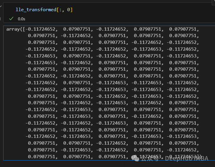
from sklearn.manifold import LocallyLinearEmbedding lle = LocallyLinearEmbedding(n_neighbors=5,n_components=1) lle_transformed = lle.fit_transform(X) plt.figure(figsize=[7, 5]) plt.scatter(lle_transformed[:, 0], np.zeros((100,1)), c=y, s=50, cmap='plasma') plt.title('First component after applying LocallyLinearEmbedding') plt.xlabel('Component 1')
There are only 2 points, actually not like this, let’s print this data.
It can be seen that the data has become the same number after dimensionality reduction, so LLE is linearly separable after dimensionality reduction, but it loses information about the data.
5. Spectral Embedding
Spectral Embedding is a dimensionality reduction technique based on graph theory and spectral theory, commonly used to map high-dimensional data to low-dimensional space. Its core idea is to use the similarity structure of the data, represent data points as nodes of a graph, and obtain a low-dimensional representation through spectral decomposition of the graph.
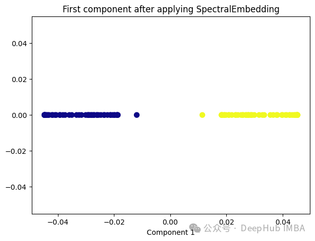
from sklearn.manifold import SpectralEmbedding sp_emb = SpectralEmbedding(n_components=1, affinity='nearest_neighbors') sp_emb_transformed = sp_emb.fit_transform(X) plt.figure(figsize=[7, 5]) plt.scatter(sp_emb_transformed[:, 0], np.zeros((100,1)), c=y, s=50, cmap='plasma') plt.title('First component after applying SpectralEmbedding') plt.xlabel('Component 1')
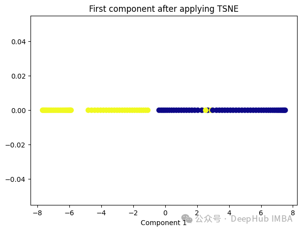
6. t-Distributed Stochastic Neighbor Embedding (t-SNE)
The main goal of t-SNE is to preserve the local similarity relationships between data points while maintaining these relationships in low-dimensional space, while trying to preserve the global structure.
from sklearn.manifold import TSNE tsne = TSNE(1, learning_rate='auto', init='pca') tsne_transformed = tsne.fit_transform(X) plt.figure(figsize=[7, 5]) plt.scatter(tsne_transformed[:, 0], np.zeros((100,1)), c=y, s=50, cmap='plasma') plt.title('First component after applying TSNE') plt.xlabel('Component 1')
It seems that t-SNE is also not very suitable for our data.
7. Random Trees Embedding
Random Trees Embedding is a tree-based dimensionality reduction technique commonly used to map high-dimensional data to low-dimensional space. It utilizes the idea of Random Forest by constructing multiple random decision trees to achieve dimensionality reduction.
The basic workflow of Random Trees Embedding:
-
Build a collection of random decision trees: First, construct multiple random decision trees. Each tree is trained by randomly selecting subsets from the original data, which helps reduce overfitting and improve generalization.
-
Extract feature representations: For each data point, construct a feature vector by using the indices of its leaf nodes on each tree. Each leaf node represents the position of the data point on a certain branch of the tree.
-
Dimensionality reduction: Map data points to low-dimensional space using the feature vectors generated by all trees in the random forest. Dimensionality reduction techniques such as PCA or t-SNE are typically used to achieve the final dimensionality reduction process.
The advantage of Random Trees Embedding is its high computational efficiency, especially for large-scale datasets. By using the idea of random forests, it can handle high-dimensional data well and does not require much tuning.
RandomTreesEmbedding uses high-dimensional sparsity for unsupervised transformation, meaning that the data we ultimately obtain is not a continuous value but a sparse representation. Therefore, no code demonstration will be provided here; interested readers can check sklearn’s sklearn.ensemble.RandomTreesEmbedding.
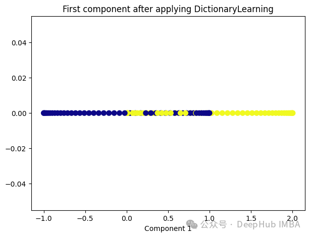
8. Dictionary Learning
Dictionary Learning is a technique used for dimensionality reduction and feature extraction, primarily for handling high-dimensional data. Its goal is to learn a dictionary composed of a set of atoms (or basis vectors) that are linear combinations of the data. By learning such a dictionary, high-dimensional data can be represented as a more compact sparse linear combination in a low-dimensional space.
One of the advantages of Dictionary Learning is that it can learn interpretable atoms, which can provide important insights into the structure and features of the data. Additionally, Dictionary Learning can produce sparse representations, leading to more compact data representations, which helps reduce storage costs and computational complexity.
from sklearn.decomposition import DictionaryLearning dict_lr = DictionaryLearning(n_components=1) dict_lr_transformed = dict_lr.fit_transform(X) plt.figure(figsize=[7, 5]) plt.scatter(dict_lr_transformed[:, 0], np.zeros((100,1)), c=y, s=50, cmap='plasma') plt.title('First component after applying DictionaryLearning') plt.xlabel('Component 1')
9. Independent Component Analysis (ICA)
Independent Component Analysis (ICA) is a statistical method for blind source separation, commonly used to estimate original signals from mixed signals. In the fields of machine learning and signal processing, ICA is often used to solve the following problems:
-
Blind source separation: Given a set of mixed signals, where each signal is a linear combination of a set of original signals, the goal of ICA is to separate the original signals from the mixed signals without knowing the specific details of the mixing process in advance.
-
Feature extraction: ICA can be used to discover independent components in the data, extracting the underlying structure and features of the data, typically used in dimensionality reduction or preprocessing.
The basic assumption of ICA is that the components in the mixed signals are statistically independent, meaning their statistical properties are independent. This is different from principal component analysis (PCA), which assumes that components are orthogonal rather than independent. Therefore, ICA is often more suitable than PCA for discovering independent components with non-Gaussian distributions.
from sklearn.decomposition import FastICA ica = FastICA(n_components=1, whiten='unit-variance') ica_transformed = dict_lr.fit_transform(X) plt.figure(figsize=[7, 5]) plt.scatter(ica_transformed[:, 0], np.zeros((100,1)), c=y, s=50, cmap='plasma') plt.title('First component after applying FastICA') plt.xlabel('Component 1')
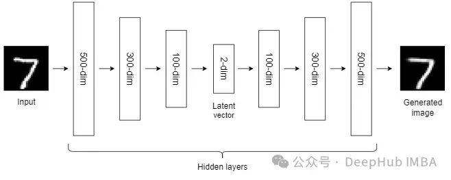
10. Autoencoders (AEs)
So far, the NLDR techniques we have discussed belong to the category of general machine learning algorithms. Autoencoders are a type of NLDR technique based on neural networks, which can handle large nonlinear data well. When the dataset is small, the performance of autoencoders may not be very good.
We have introduced autoencoders many times, so we will not elaborate on them here.
Conclusion
Nonlinear dimensionality reduction techniques are a class of methods used to map high-dimensional data to low-dimensional space, usually suitable for cases where the data has a nonlinear structure.
Most NLDR methods are based on nearest neighbor methods, which require all features in the data to be on the same scale, so if the scales of the features differ, scaling is also needed.
Additionally, these nonlinear dimensionality reduction techniques may exhibit different performance across different datasets and tasks, so when choosing the appropriate method, factors such as data characteristics, dimensionality reduction goals, and computational resources need to be considered.
Editor: Wang Jing