Thorough Understanding of RNN (Recurrent Neural Networks)

This article is a bit long, and I will divide it into several parts. Through this article, I hope to help you thoroughly understand the principles of RNN (Recurrent Neural Networks) and be able to implement it at the code level.

Table of Contents

1. What This Article Does
2. Inputs and Outputs of RNN
3. RNN Network Structure
4. Generating Datasets
5. A Brief Taste of RNN Layer Forward Propagation
6. Code Implementation

1 What This Article Does

Through this article, I created a demo. We know that RNN is used to process sequential data, which needs to consider the temporal relationships between values in the sequence, or the relationships between preceding and following values.

In order to verify that my model can indeed learn the relationships between sequences from a more intuitive perspective during the learning process, I generated a series of virtual sequences, which have very strong internal regularities.

“What Data Was Generated”

This data series has a length of 1000, and the element types only include 20, which are the numbers from 0 to 19. Here’s a small example.

0, 1, 2, 3, 4

2, 3, 4, 5, 6

15, 16, 17, 18, 19

5, 6, 7, 8, 9

When generating this very long data series, I first randomly generated a number as the starting point, and then generated a series of continuous values starting from this point to append to the end of the sequence data. For example, there are four such groups of data above. These data should be a string rather than line by line, so they should look like this.

0, 1, 2, 3, 4, 2, 3, 4, 5, 6, 15, 16, 17, 18, 19, 5, 6, 7, 8, 9

Thus, the internal regularity of this sequence data is very obvious; the pattern is that the number that should appear after a number can be found. This string of data indeed conforms to such a pattern, but this pattern does not hold everywhere. Even in real life, sequences have such characteristics where the current value is related to the previous value, but sometimes the relationship is strong, and sometimes it is weak.

In the later sections, I will use code to generate this string of data. Of course, the length of this string of data is definitely not just this; the sequence length generated in this article is 1000.

“What the Model Should Learn”

Since the manually created data presents such a pattern, we hope our model can learn this pattern.

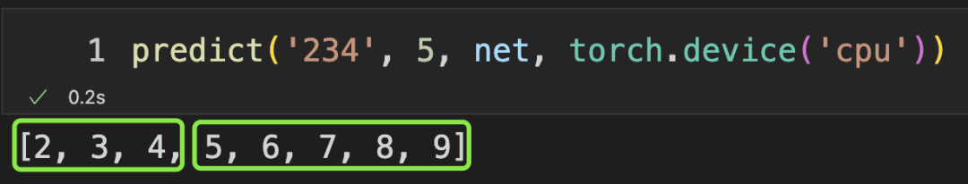
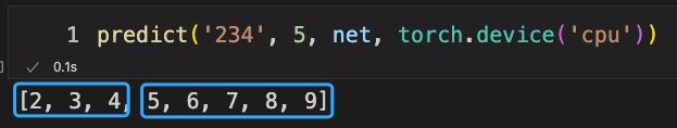
Finally, I hope that given a prefix like 234, the model can predict five subsequent characters, and the model should return a string of data like 23456789.

After training the model, it indeed achieved this expected effect, allowing us to see the changes produced by the model after training in an intuitive way during the learning process.

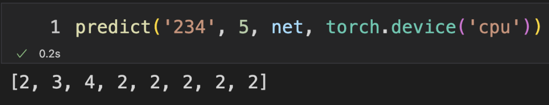
Before training the model, predictions were made using default parameters, and we can see that the results were unsatisfactory.

2 Inputs and Outputs of RNN

Based on the above content, I hope this network structure can take a prefix as input and output the most likely subsequent values.

So, besides inputting the entire prefix at once into the network, are there any other methods? Of course, there are! We can also choose to input one value into the network at a time, and then input the second value. At this time, we hope the network has a certain memory function and can remember that the second value was input after the first value.

Every time we input into the network, it will produce an output based on the current inputs.

For example:

When I input the first value, the network produces an output based on this unique input.

When I input the second value, the network produces another output based on both the first and the second values inputted.

“Single-step Prediction”

If the prefix only has two values 23, inputting 2 and 3 into the network at once will allow the memory function to produce an output value that is the most likely first value to appear after 23. This completes the single-step prediction.

“Multi-step Prediction”

Based on single-step prediction, we can predict what the first value that appears after 23 is. If we take the predicted value as input to the network again, we will get an output, and at this point, we have obtained the two most likely values to appear after 23. This completes the two-step prediction. If you want to predict a longer string, you can continue to repeat the previous steps to complete multi-step predictions.

“What Is the Input”

We keep saying to input a value, but what exactly is this input value? For example, for a prefix 234, according to the previous logic, I should first input 2 into the network, then 3, and finally 4. When I input 4 into the network, the output value provided by the network will be the most likely next value based on 234.

When I input 2 into the network, am I really inputting 2? Not really.

The value input into the network is the one-hot encoding corresponding to the number 2. In fact, one-hot encoding can be understood as a probability distribution. (Don’t worry, even the seemingly obscure concepts will be clarified, just knowing this is enough for now.)

“What Is the Output”

You can imagine that when inputting 2 into the network, what is input is the one-hot encoding of the value 2. At this time, you hope the network provides the next value that appears after the number 2. However, the network does not output a single value directly; instead, it outputs a probability distribution. (Again, don’t worry.)

“What Does Probability Distribution Mean”

In the virtual data we constructed, there are a total of categories, which are the integers that make up the sequence data.

For convenience in examples, I will reduce the categories here and only use six integers from 0 to 5 as all possible values in the sequence data.

If we want to input the number 2 into the model to predict what the next possible value is, then in the case of six possible values, the one-hot encoding corresponding to 2 is as follows.

You can see that the one-hot encoding for 2 has a 1 only at the second position, while all other positions are 0. (Here, the vector index starts from 0.)

Thus, you can understand this encoding as a probability distribution, indicating that for the second value, which is 2, the probability is 1, while the probabilities for other positions are 0. Therefore, we express a value through a probability distribution. The model’s output is also like this.

“The Model Is a Black Box”

You can temporarily think of the network model as a black box whose internal structure is unknown. As long as you provide input, it will produce output. Let’s assume this black box looks like this.

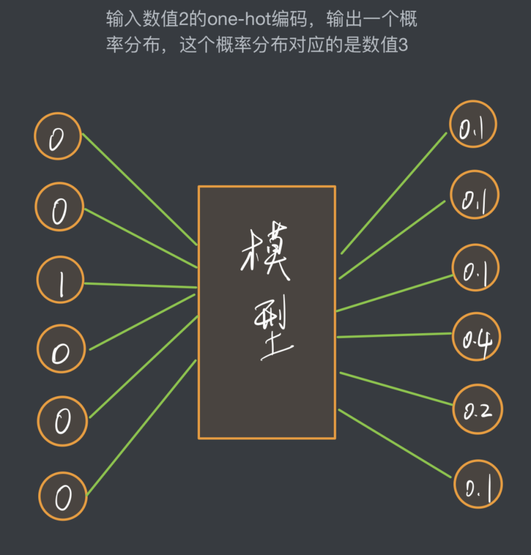
Through the output probability distribution, we can know that after the prediction of this model, the next most likely value to appear is the third value (which is 3), because it corresponds to the highest probability, while the probabilities for other values are lower.

3 RNN Network Structure

In the previous content, we have already understood what the inputs and outputs of the RNN network look like for our example.

Now let’s take a look at what this network structure specifically looks like.

“MLP Network Structure”

This is a multi-layer perceptron model, which can be expressed as follows.

Given a small batch of samples and weight parameters

1. is a matrix, each row is a one-hot encoding of a value. For convenience of understanding, imagine it as a sample matrix with only rows; treat it as a row vector.
2. is a weight matrix, where represents the number of hidden units in this layer.
3. , used to represent the output of the hidden layer. Since the sample size is and the number of units in this layer is , there are columns, indicating that the output dimension of this hidden layer is , and it simultaneously processes samples, resulting in rows. Of course, you can also analyze the shape of the matrix from a purely mathematical perspective.
4. The function represents the activation function.
5. is a weight matrix, we use a linear layer as the output layer, which can control the output dimension of the output layer. You can see that the output layer has no activation function.
6. represents the final output of the output layer.
7. are the biases corresponding to the layers, and both of these vectors are row vectors. Vectors and matrices cannot perform addition, but here the broadcasting mechanism is used, and the number of columns of the matrix to be summed is the same as that of this vector, so through the broadcasting mechanism, this vector will be added to each row of the matrix, resulting in the final result.

So, what is the problem now? For the structure of , it has no memory function. Every time a new sample is input, it does not remember what was previously input.

“Introducing Memory Function”

In the matrix, indeed, each row is a one-hot encoding of a value.

You should know the concept of time steps; you can understand this concept by referring to this article.

Portal: The Simplest Sequence Model – Part One

If this matrix represents that in the matrix, there are three samples, and most importantly, these three samples are values located at the same time step.

If the time step is . Through the sequence, we constructed such three segments. In this sequence, each row is a sample, which seems contradictory to what was said earlier. (Let me explain slowly.)

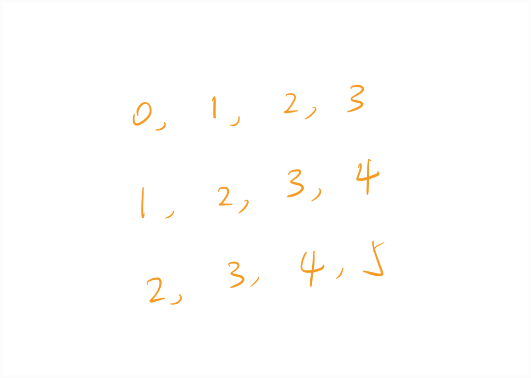
The matrix contains samples, and each row is merely a one-hot encoding of a value, while the values shown above each row contain multiple values.

The matrix stores samples at a specific moment, only storing the samples at a specific time step, not all time steps. The three rows shown above contain the corresponding values of this sample at all time steps.

Our model only inputs values at one time step, not all values corresponding to all time steps of this sample at once.

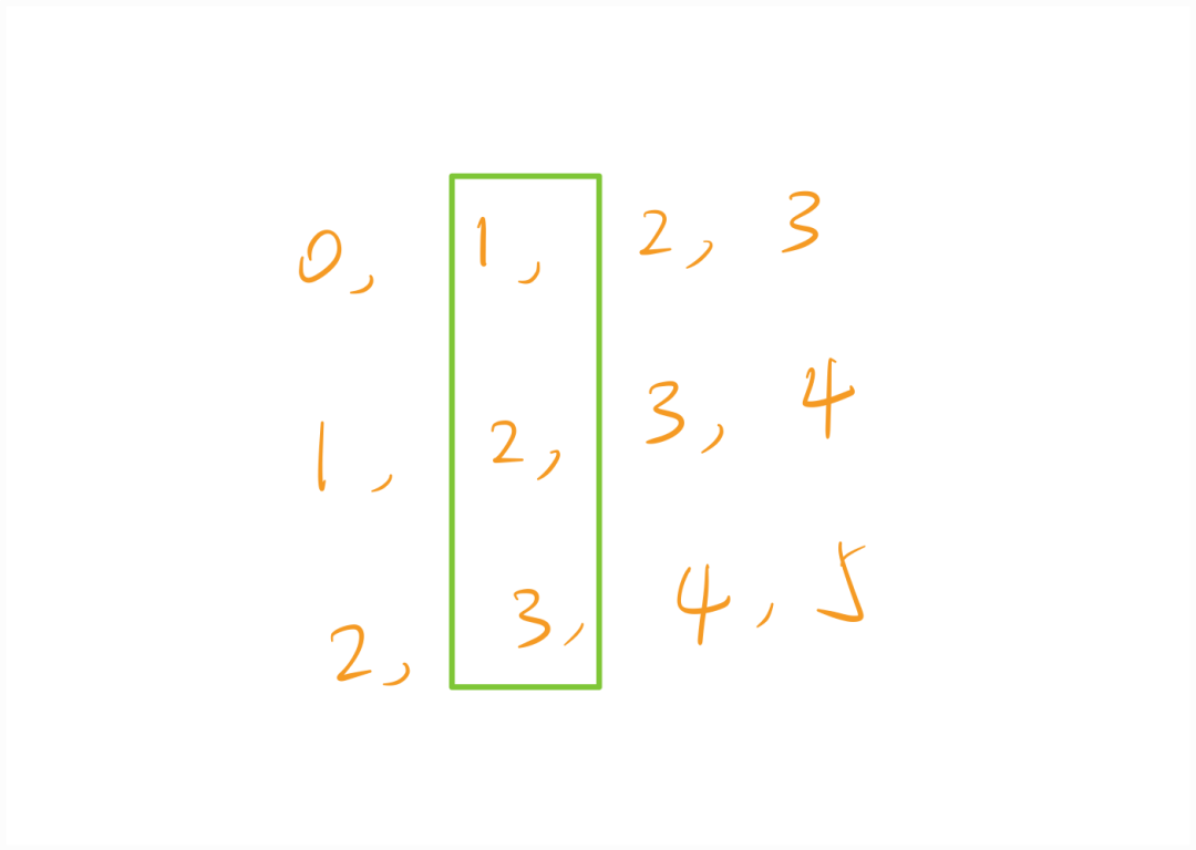
If we start counting from time steps, now the values corresponding to each sample at the moment are those marked in the green box. If we want to batch process multiple samples at once, the matrix should look like this. (The selectable value types are still six, from 0 to 5.)

The first row of this matrix corresponds to the one-hot encoding of the value corresponding to the first sample at time step 1. The subsequent values follow suit.

Note that the model cannot input all values of a sample corresponding to all time steps into the network at once, but it can input multiple samples at once; these multiple samples only contain the values of these samples at a specific time step, not the values at all time steps. According to the properties of matrix operations, this achieves the goal of batch processing.

Explaining this is to clarify the meaning of adding a superscript to the upper right corner of the matrix.

“Note”

The matrix represents the sample formed by this sample at time steps. For other matrices, if I add a superscript in the upper right corner, it indicates that this sample is computed from the input.

Alright, how do we introduce the memory function?

We just need to slightly modify the structure.

You can see that in this network structure, we have only added one item, thus giving this network structure memory functionality.

Don’t worry! This is just the output value of the hidden layer computed when we input! It’s really just that! There’s nothing magical about it!

Then, when we input into the network, we also need to input it together. This seems to contain the information we previously input into the network. Looking at it this way, doesn’t it seem like it has a bit of memory?

Let’s take another look at the calculation of the hidden layer:

You can see that it sums the content produced at time step and the content produced at time step. This is like adding the information from this time and the past together.

You can see I’ve been saying it’s like this or that. Because current neural network models indeed cannot be well explained. A friend of mine told me that this thing is like a mysterious concept. It does seem to be the case. However, from an intuitive perspective, we can still assign some meaning to understand it.

So, our network structure actually becomes two types of inputs, which are

1. The sample matrix at time step.
2. The hidden state matrix.

And the model’s output also needs to change to two types, which are

1. The probability distribution corresponding to each input sample, which is the matrix.
2. And the output produced by the hidden layer in this computation.

If you have to represent it with a diagram:

The superscript in the upper right corner is placed at the lower right position; just understand it like that.

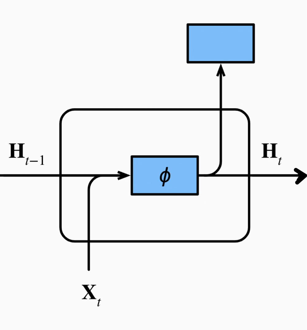
Because we need to use it for the next round of input, the output of the hidden layer is useful for us later, so we must also return the output of the hidden layer when writing the program, making it convenient for the next input.

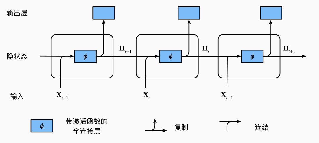
So now you understand why it’s called a recurrent neural network, right?

You notice that for the sample matrix at different time steps, the weight matrices used during forward propagation have always been the same and have not changed! Moreover, every time, the output from the last time is used as input for the next time. This process is like a loop. And when you predict multiple steps, you are also looping this operation.

If we draw the process of repeatedly inputting and outputting into a diagram and connect them, it can look like this. Be sure to note that the weight parameters used each time are the same; you can look at this diagram from left to right.

“Where Does the Hidden State Come From”

Do you wonder where the hidden state matrix comes from when you have to input the hidden state matrix every time you input the sample matrix? When you input the sample matrix for the first time, since no hidden state matrix has been generated yet, where does this hidden state matrix come from?

This question is easy to solve: when you input content into the model for the first time, there is no information, so the sample matrix is a full matrix. Therefore, when performing this operation, the added matrix is also a full matrix, which means no prior information is accumulated.

“How to Measure Loss”

The process of training the model is nothing more than optimizing the loss function. And how do we measure the loss?

Recall that our model predicts the next value, outputting a probability distribution. Now, we have a training dataset, and during training, we certainly know what the input value is and what the corresponding next value should be.

Therefore, we should find a way to compare the output probability distribution with the probability distribution corresponding to the next value (which is the one-hot encoding corresponding to the next value) to see how large the difference is.

This operation is very straightforward; cross-entropy can measure the difference between two probability distributions. Therefore, we can choose cross-entropy as the loss function. In this way, we have resolved all theoretical issues.

As for cross-entropy, I won’t elaborate here.

4 Generating Datasets

“One-hot Encoding”

import torch
import torch.nn.functional as F

vec = torch.arange(3)
F.one_hot(vec, num_classes=5)  # Number of classes is 5

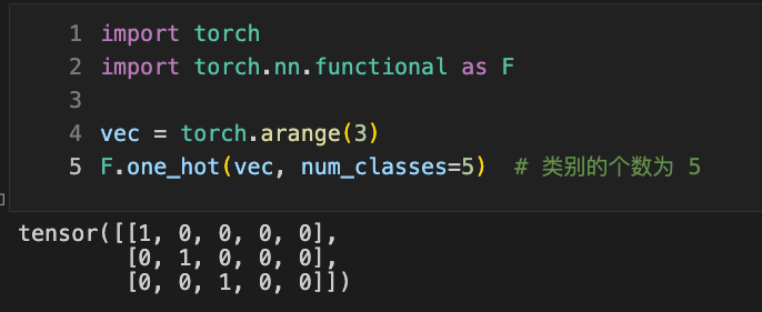
Create a vector and perform one-hot encoding on it. Each element in this vector will be expanded into a vector, thus adding an extra dimension and turning it into a matrix.

“One-hot Encoding for Matrices”

mat = torch.tensor([
    [1, 2, 3],
    [4, 5, 6]
])

# batch_size, num_steps,  num_classes
mat1 = F.one_hot(mat, 7)
print(mat1.shape)

# num_steps, batch_size, num_classes
# Each time we get all samples' data at the same time step
mat2 = F.one_hot(mat.T, 7)
print(mat2.shape)

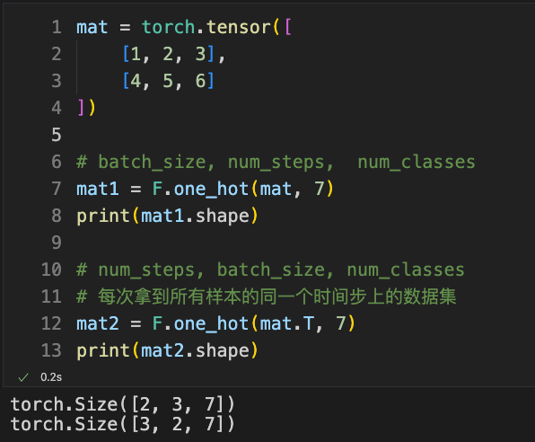
Create a matrix, treating this matrix as having 2 samples, each with a time step of 3.

1. First, look at the first print statement; we directly perform one-hot encoding on it. At this point, an additional third dimension is added to the 2-row 3-column matrix. How to view this matrix? It becomes a 3-row 7-column matrix, representing the one-hot encoding of all values of the 0th sample. The vector is the one-hot encoding of the value corresponding to the 0th time step of the 0th sample, and so on.
2. Now, let’s look at the second print statement. When we compute it, we first transpose the matrix and then perform one-hot encoding. The shape of the matrix was number of samples × time step length, but after transposing, it becomes time step length × number of samples. I use to represent the transposed matrix, which means the vector formed by the values corresponding to the 0th time step of all samples. Then I perform one-hot encoding on it, and again an additional dimension is added. At this point, represents the matrix obtained from the one-hot encoding of all values corresponding to the 0th time step of all samples. It’s just like what we saw in the formulas; however, here, it’s actually the matrix. Similarly, represents the matrix.

“Generating Random Sequence Data”

Since we want to generate a sequence of length, and each time generate numbers, we need to generate times.

Each time we generate a number, first randomly select a starting point, then append a number of values starting from this point to the list seq.

from random import randint

seq = []

for i in range(100):
    # Each time generate a continuous sequence of length 10
    start = randint(0, 10)  # Randomly select a number in the closed interval [0, 10]
    for j in range(start, start+10):
        seq.append(j)

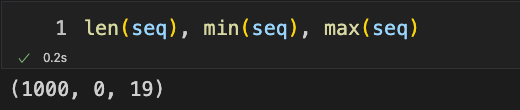
You can see that the length is , with the minimum value being and the maximum value being.

“Constructing the Dataset”

Now we have only generated this string of values, but it cannot be used directly; we need to construct it into a sample matrix. If you do not understand this operation in detail, you can refer to this article’s data construction method.

Portal: The Simplest Sequence Model – Part One

The data construction method differs slightly from the method constructed in the article above. In the code below, the construction is equivalent to but slightly different.

T = len(seq)  # Length of sequence data seq
num_steps = 20  # Length of time steps
num_classes = 20  # How many types of tokens; used for generating one-hot encoding

dtype = torch.int64

x = torch.tensor(seq, dtype=dtype)
X = torch.zeros((T-num_steps, num_steps), dtype=dtype)
Y = torch.zeros((T-num_steps, num_steps), dtype=dtype)

for i in range(num_steps):
    X[:, i] = x[i:T-num_steps+i]
    Y[:, i] = x[i+1:T-num_steps+i+1]

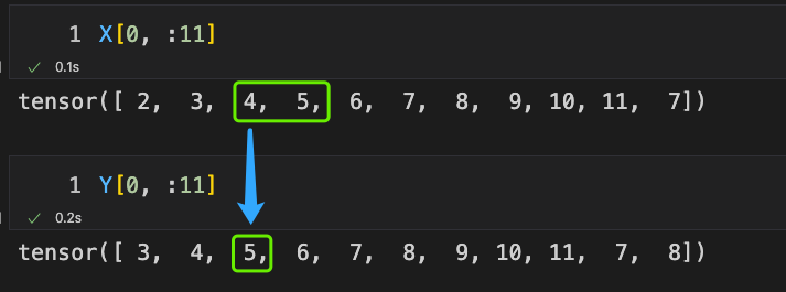
Let’s take a closer look at these two lines of code:

X[:, i] = x[i:T-num_steps+i]
Y[:, i] = x[i+1:T-num_steps+i+1]

After reading the article The Simplest Sequence Model - Part One, this construction should be easy to understand. However, there is a slight difference in the construction; that is, when slicing, both the starting and ending positions of the slices are increased by in comparison to the base.

This means that the expected output for inputting a value into the model should be . Since we predict by using the previous value in the sequence to predict the next possible value, we just need to shift the sequence backwards by one position during construction.

Similarly, you can verify that:

5 should appear after 4, and indeed, the same position in the matrix satisfies this requirement.

“Creating Data Iterators”

Select the batch size, and to ensure that all sample data generated by the iterator have the same batch size, we only need to generate sample_epochs small batches. To maintain the batch size of each generated batch, we divide the total number of samples by the batch size of 50 and take the floor to get sample_epochs.

Thus, we only select the first num_samples samples from the sample matrix to construct the data iterator.

batch_size = 50  # Batch size

sample_epochs = X.shape[0] // batch_size
num_samples = sample_epochs * batch_size

from torch.utils import data
dataset = data.TensorDataset(X[:num_samples, :], Y[:num_samples, :])
diter =data.DataLoader(dataset=dataset, batch_size=batch_size)

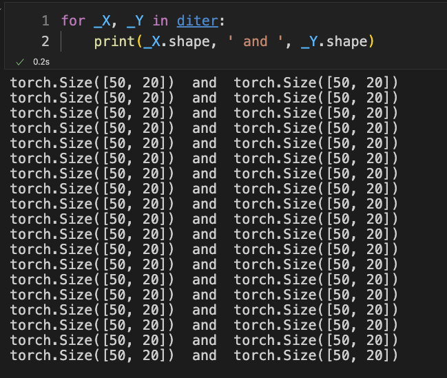
for _X, _Y in diter:
    print(_X.shape, ' and ', _Y.shape)

You can see that the shape of each generated small batch of data is .

5 A Brief Taste of RNN Layer Forward Propagation

import torch
from torch import nn
import torch.nn.functional as F

num_hiddens = 256  # Number of outputs in RNN hidden layer - also the number of hidden units
num_classes = 20  # Number of inputs in RNN hidden layer - also the length of one-hot encoding - represents the number of types of tokens

# Input is num_classes
# Output is num_hiddens
# 1 layer of RNN stacked
rnn_layer = nn.RNN(num_classes, num_hiddens, 1)

We can directly use to create a layer. Here, the layer refers specifically to the hidden layer in the model that contains the activation function.

Let’s take a look at the specific parameters:

1. The first parameter num_classes passed to nn.RNN specifies the length of the data input to the RNN layer each time, and we are inputting the length of a one-hot encoded vector, which in this case is 20.
2. The second parameter num_hiddens passed to nn.RNN specifies the number of units in the layer (the number of neurons), and it also represents the output dimension of the layer.
3. The third parameter passed to nn.RNN is 1, indicating that only one layer of RNN is stacked. You can imagine that we can also use the output value as input for the next layer, but we do not intend to do that here; we will only use one layer.

“Creating the Hidden State”

When performing forward propagation with the layer, in addition to inputting samples, we also need to input a hidden state. We can directly initialize a matrix filled with zeros as the hidden state.

# size = (number of hidden layers, batch size, number of neurons)
# In the following test, it only contains 1 data sample
state = torch.zeros(size=(1, 1, num_hiddens))
state.shape

The shape of the generated zero matrix is as follows.

(number of hidden layers, batch size, number of neurons)

1. The number of hidden layers: this is the third parameter, as each layer requires a hidden state as input. This is easy to understand.
2. Batch size: each layer can batch process multiple samples at the same time step (multiple vectors are a matrix). The values corresponding to the previous time step and the subsequent time step of different samples are temporally and sequentially related, while there is no relation between different samples. Therefore, each sample needs a hidden state parameter, hence the second dimension is the batch size. “Note”: Here, we first use one sample and perform forward operations with default weight parameters to get a feel for how to use the layer.
3. The number of neurons: the number of neurons here is the number of units in the layer, which is also the number of output dimensions. Looking at this formula carefully, you can observe the shape of the matrix and understand why the shape is . Here, n is the batch size, and h is the number of units.

“Creating a Sample x_t”

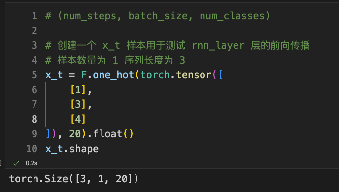
After understanding the above, I believe you can easily understand why we create a matrix of this shape.

# Create a sample x_t for testing the rnn_layer layer's forward propagation

# Time step length num_steps=3, sample size batch_size=1
# (num_steps, batch_size, num_classes)
x_t = F.one_hot(torch.tensor([
    [1],
    [3],
    [4]
]), 20).float()

“Forward Propagation”

Next, we just need to input x_t and the hidden state state.

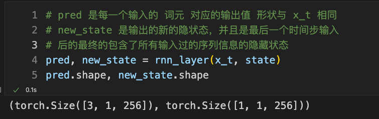
# pred is the output value corresponding to each input token, with the same shape as x_t
# new_state is the new hidden state output after the last time step input, containing all the sequence information inputted
pred, new_state = rnn_layer(x_t, state)
pred.shape, new_state.shape

It is necessary to explain the shapes of pred and new_state.

1. The shape of new_state is easy to understand; it is the same as the shape of state inputted into rnn_layer, so no further explanation is needed.
2. The shape of pred is , where 3 represents the three time steps. You can see that although we only have one sample in the sample matrix, its length is 3, which means the time step is 3. Here, 1 represents the number of samples in the sample matrix, and 256 represents the output dimension size of rnn_layer. Combined, it is a matrix representing the output produced by the value at the 0th time step input into the model (each row is an output of length 256). However, since we only input one sample, it is practically a matrix with 1 row and 256 columns. More generally, it represents the output vector of length 256 produced when the one-hot encoding of the value corresponding to the ith time step of the jth sample is input into the model.

We can further explore the values stored in pred and new_state. According to the logic inferred earlier, the content in new_state is actually the same as that in pred at the last time step.

1. represents the output of the rnn_layer layer for the 0th sample at the 2nd time step, and since the time step length of the sample is 3, the 2nd time step is the last moment. Here we only look at the first three values of this vector.
2. represents the output produced when inputting the one-hot encoding of the value corresponding to the last time step of the 0th sample into the model. Here we only look at the first three values. Note: The layer we generated contains only one layer, so it only has the 0th layer, and the sample matrix only contains one sample, so it only has the 0th sample.

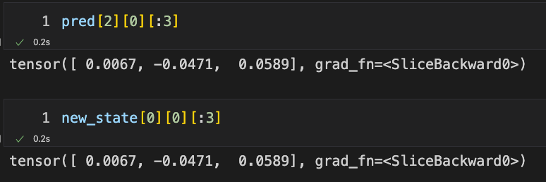
Now you can find that their values are the same. This also verifies what was said earlier.

6 Code Implementation

Now we finally arrive at the code implementation section!

For simplicity, I have directly written the code for creating the layers in the class as specific values.

class RNNModel(nn.Module):
    def __init__(self):
        super().__init__()
        
        # one-hot encoding length is 20
        # number of hidden units
        # number of layers stacked in rnn
        self.rnn = nn.RNN(20, 256, 1)

        # Use a linear layer to convert it into a probability distribution output
        self.linear = nn.Linear(256, 20)

    def forward(self, inputs, state):
        # First perform one-hot encoding on the input batch sample matrix
        X = F.one_hot(inputs.T.long(), 20)
        X = X.to(torch.float32)
        
        Y, state = self.rnn(X, state)
        output = self.linear(Y.reshape(-1, Y.shape[-1]))
        return output, state

    def begin_state(self, batch_size):
        # Number of stacked rnn layers, batch size, number of hidden units
        return torch.zeros(size=(1, batch_size, 256))

1. The forward function defines the forward propagation logic.
2. The begin_state function initializes a state.

One important operation is the line in the forward function that computes output with Y.reshape(-1, Y.shape[-1]). Here, Y.shape[-1] is the length of the one-hot vector. After this reshape, the shape of the resulting matrix is number of time steps × batch size rows and 256 columns.

How should this shape be understood?

1. 256 columns are easy to understand, because for a one-hot vector as input to the model, the layer will produce 256 outputs, meaning that each row of the matrix obtained after reshape is an output.
2. number of time steps × batch size rows represent the number of outputs. Each sample has number of time steps values, and there are batch size samples. Thus, the number of inputs is also number of time steps × batch size. The layout of the matrix after reshape also needs to be understood. “1)” It will sequentially place the output of the 0th sample at the 0th time step in the first row, then the output of the 1st sample at the 0th time step in the second row, until all outputs at the 0th time step are sequentially arranged in each row, completing the first part. “2)” Then it will sequentially arrange the outputs of all samples at the 1st time step. Well… until all outputs across all samples at all time steps are completed, this is how to understand the layout of the matrix after reshape.

Another difference is that a linear layer has been added in the forward function; the input to the linear layer is , and the output is , which compresses the output dimension of the layer to a length of . This transforms it into a probability distribution for the values.

return output, state returns the final output and the newly produced state.

“Model Training”

Details about model training are included in the comments!

net = RNNModel()
state = net.begin_state(50)

# Use cross-entropy loss function
loss = nn.CrossEntropyLoss()

# Use SGD as the optimizer
updater = torch.optim.SGD(net.parameters(), lr=0.01)

# Iterate over all data for 100 times
for i in range(100):
    for X, Y in diter:
        
        # Flatten Y after transposing it into a vector
        # This is very similar to the output produced by forward
        # If we perform one-hot encoding on y again
        # it will match the arrangement of output in forward
        y = Y.T.reshape(-1)
        
        # Reset state to zero when starting to discuss a new small batch of data
        # Because the current small batch of data has no relation to the previous batch
        state = net.begin_state(batch_size=batch_size)
      
        # Generate predictions y_hat and new state
        y_hat, state = net(X, state)
        
        # Here, the loss passed to y_hat is a probability distribution
        # The loss will automatically perform one-hot encoding on y.long()
        # and compute the cross-entropy loss between y_hat and y.long()
        l = loss(y_hat, y.long()).mean()
        updater.zero_grad()
        l.backward()
        updater.step()
        
        # Output the loss on the small batch of data
        print(l)

We can see that the loss is decreasing:

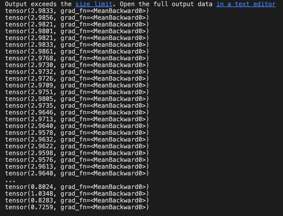
You can also calculate how the loss changes for the entire dataset by adjusting the learning rate and the number of iterations to see the optimization effect.

“How to Predict”

def predict(prefix, num_preds, net, device):  #@save
    """
    Generate new characters after the prefix
    num_preds: How many values to generate subsequently
    net: Your model
    device: Whether to compute using cpu or gpu
    """
    # batch_size = 1 ==> Predict for one string
    state = net.begin_state(batch_size=1)
    outputs = [int(prefix[0])]  # Place the numeric type of prefix[0] into outputs
    
    # get_input function, each time takes a value from the end of outputs
    # then shapes it into a form that can be input into the net model and returns
    get_input = lambda: torch.tensor([outputs[-1]], device=device).reshape((1, 1))
    
    for y in prefix[1:]:  
        # Warm-up period ==> Initialize the information from prefix into state
        # y starts taking values from the 1st element of prefix
        # When y takes prefix[1], the input obtained from get_input() is prefix[0]
        # which just happens to be offset, and there’s no problem
        # The reason state is also an input parameter for the network
        # is to use state to retain the information of the prefix
        # This allows the network to remember all the prefix information
        # during prediction, rather than predicting based solely on prefix[-1]
        inputs = get_input()
        _, state = net(inputs, state)
        outputs.append(int(y))

    # From here, start predicting the characters following the prefix
    # Each time, the last output value is used as the next input value
    # The last output value is a value at one time step, not a sequence
    # But don't worry, the new information input into the network earlier
    # is all stored in the state
    for _ in range(num_preds):  # Predict num_preds steps
        y, state = net(get_input(), state)
        outputs.append(int(y.argmax(dim=1).reshape(1)))

    # Convert the index values to their corresponding tokens (here characters)
    return outputs

“Prediction”

predict('234', 5, net, torch.device('cpu'))